import matplotlib
from matplotlib import pyplot

import numpy as np

from common import draw_classic_axes, configure_plotting

configure_plotting()

pi = np.pi
  

Solutions for lecture 7 exercises

Warm up exercises

1. Check by yourself

2. $$[v_g]=\frac{[E]}{[p]}=\frac{m}{s}$$

3. $$[m^{\ast }]=\frac{[p^2]}{[E]}=kg$$

4.

$$m^{\ast }=m_e,$$ where $m_e$ is the free electron mass. This is expected because the free elctrons are not subject to a potential

5. If the dispersion relation is parabolic, so in the free electron model.

Exercise 1: Lattice vibrations

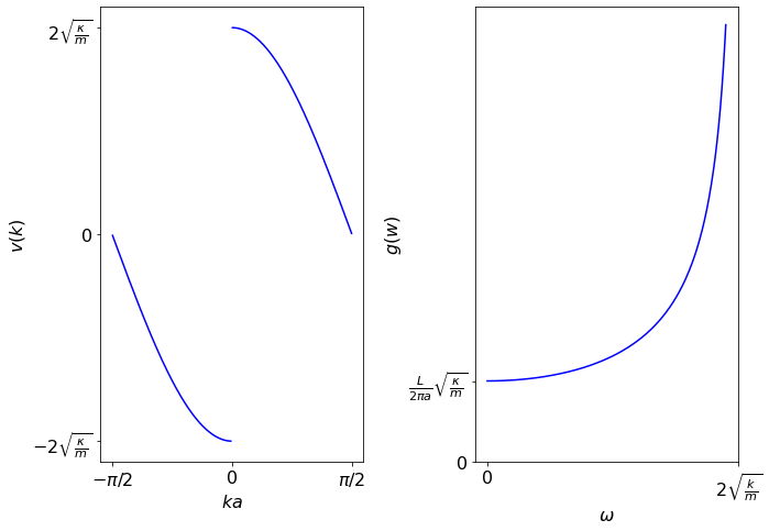
1. The group velocity is given by $$\begin{array}{rlr}{v}_g(k)& =\frac{\partial \omega (k)}{\partial k}& =a\sqrt{\frac{\kappa }{m}}\cos (\frac{ka}{2})\frac{\sin (ka/2)}{|\sin (ka/2)|},\end{array}$$ which can be written as $$v_g=a\sqrt{\frac{\kappa }{m}}\{\begin{array}{lll}& \cos (\frac{ka}{2}),0<ka<\pi & -\cos (\frac{ka}{2}),-\pi <ka<0\end{array}$$

2. The density of states is $$\begin{array}{rlrlr}g(\omega )& =\frac{L}{\pi }\left|\frac{1}{v_g}\right|& =\frac{L}{a\pi }\sqrt{\frac{m}{\kappa }}\frac{1}{\cos (ka/2)}& =\frac{L}{a\pi }\sqrt{\frac{m}{\kappa }}\frac{1}{\sqrt{1-{\sin }^2(ka/2)}}& =\frac{2L}{a\pi }\frac{1}{\sqrt{4\kappa /m-{\omega }^2}},\end{array}$$ where we substituted back the dispersion relation.

3.

pyplot.subplot(1,2,1)
k = np.linspace(-pi+0.01, pi-0.01, 300)
pyplot.plot(k[0:149], np.sin(k[0:149])/(np.sqrt(1-np.cos(k[0:149]))),'b');
pyplot.plot(k[150:300], np.sin(k[150:300])/(np.sqrt(1-np.cos(k[150:300]))),'b');
pyplot.xlabel(r'\(ka\)'); pyplot.ylabel('\(v(k)\)');
pyplot.xticks([-pi, 0, pi], [r'\(-\pi/2\)', 0, r'\(\pi/2\)']);
pyplot.yticks([-np.sqrt(2), 0, np.sqrt(2)], [r'\(-2\sqrt{\frac{\kappa}{m}}\)', 0, r'\(2\sqrt{\frac{\kappa}{m}}\)']);
pyplot.tight_layout();

pyplot.subplot(1,2,2)
w = np.linspace(0, 0.95, 300);
g = 1/np.sqrt(1-w**2);
pyplot.plot(w, g, 'b');
pyplot.xlabel(r'\(\omega\)'); pyplot.ylabel('\(g(w)\)');
pyplot.xticks([0, 1], [0, r'\(2\sqrt{\frac{k}{m}}\)']);
pyplot.yticks([0.5, 1], [0, r'\(\frac{L}{2\pi a}\sqrt{\frac{\kappa}{m}}\)']);
pyplot.tight_layout();

4.

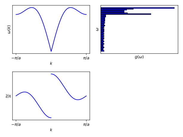
Hint: The group velocity is given as $v=\frac{d\omega }{dk}$, draw a coordinate system under or above the dispersion graph with $k$ on the x-axis in which you draw $\frac{d\omega }{dk}$. Draw a coordinate system next to the dispersion with $g(\omega )$ on the y-axis in which you graph $(\frac{d\omega }{dk}{)}^{-1}$.

Plots

Exercise 2: Vibrational heat capacity of a 1D monatomic chain

1.

For the energy we have: \($⟨E⟩=\int \hslash \omega g(\omega )(n_{BE}(\hslash \omega )+\frac{1}{2})d\omega$\) with $g(\omega )$ being the DOS calculated in exercise 1 and $n_{BE}(\hslash \omega )=\frac{1}{e^{\hslash \omega /k_{B}T}-1}$.

2.

For the heat capacity we have: \($C=\frac{d⟨E⟩}{dT}=\int g(\omega )\hslash \omega \frac{d{n}_{BE}(\hslash \omega )}{dT}d\omega$\)

Exercise 3: Next-nearest neighbors chain

1.

The Schrödinger equation is given by: $|\mathrm{\Psi }⟩=\sum _n{\varphi }_n|n⟩$ such that we find $$E{\varphi }_n=E_0{\varphi }_n-t{\varphi }_{n-1}-t{\varphi }_{n+1}-t^{\prime }{\varphi }_{n-2}-t^{\prime }{\varphi }_{n+2}$$

2.

Solving the Schrödinger equation yields dispersion: \($E(k)=E_0-2t\cos (ka)-2t^{\prime }\cos (2ka)$\)

3.

$$m^{\ast }=\frac{{\hslash }^2}{2a^2}\frac{1}{t\cos (ka)+4t^{\prime }\cos (2ka)}$$

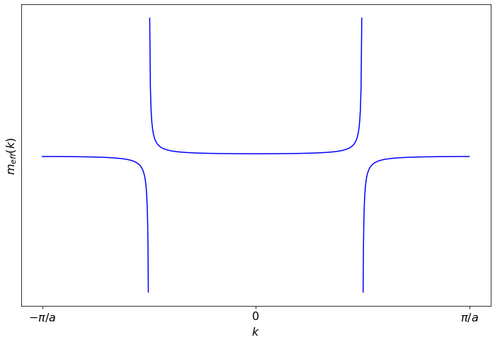
Plot for t=t':

k1 = np.linspace(-pi, -pi/2-0.01, 300);
k2 = np.linspace(-pi/2+0.01, pi/2-0.01, 300);
k3 = np.linspace(pi/2+0.01, pi, 300);

pyplot.plot(k1, 1/(5*np.cos(k1)),'b');
pyplot.plot(k2, 1/(5*np.cos(k2)),'b');
pyplot.plot(k3, 1/(5*np.cos(k3)),'b');
pyplot.xlabel(r'$k$'); pyplot.ylabel('$m_{eff}(k)$');
pyplot.xticks([-pi,0,pi],[r'$-\pi/a$',0,r'$\pi/a$']);
pyplot.yticks([],[]);
pyplot.tight_layout();

4.

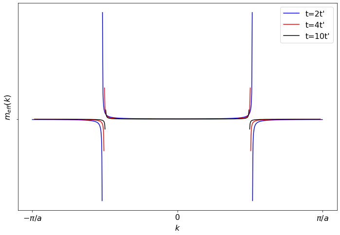
Plots for 2t'=t, 4t'=t and 10t'=t:

def m(k,t):
    return 1/(np.cos(k)+4*t*np.cos(2*k))

k1 = np.linspace(-1.6, -0.83, 300);
k2 = np.linspace(-0.826, 0.826, 300);
k3 = np.linspace(0.83, 1.6, 300);

pyplot.plot(k1, m(k1,2),'b');
pyplot.plot(k2, m(k2,2),'b');
pyplot.plot(k3, m(k3,2),'b',label='t=2t\'');
pyplot.xlabel('$k$'); pyplot.ylabel('$m_{eff}(k)$');
pyplot.xticks([-1.6,0,1.6],[r'$-\pi/a$',0,r'$\pi/a$']);
pyplot.yticks([0],[]);
pyplot.tight_layout();

k1 = np.linspace(-1.58, -0.81, 300);
k2 = np.linspace(-0.804, 0.804, 300);
k3 = np.linspace(0.81, 1.58, 300);

pyplot.plot(k1, m(k1,4),'r');
pyplot.plot(k2, m(k2,4),'r');
pyplot.plot(k3, m(k3,4),'r',label='t=4t\'');

k1 = np.linspace(-1.575, -0.798, 300);
k2 = np.linspace(-0.790, 0.790, 300);
k3 = np.linspace(0.798, 1.575, 300);

pyplot.plot(k1, m(k1,10),'k');
pyplot.plot(k2, m(k2,10),'k');
pyplot.plot(k3, m(k3,10),'k',label='t=10t\'');

pyplot.legend();