    import matplotlib.pyplot as plt

import numpy as np
from math import sqrt,pi

from common import draw_classic_axes, configure_plotting

from plotly.subplots import make_subplots
import plotly.graph_objs as go

configure_plotting()
Lecture 9 – Crystal structure
based on chapter 12 of the book
Expected prior knowledge
Before the start of this lecture, you should be able to:
- use elementary vector calculus
Learning goals
After this lecture you will be able to:
- Describe any crystal using crystallographic terminology, and interpret this terminology
- Compute the volume filling fraction given a crystal structure
- Determine the primitive, conventional, and Wigner-Seitz unit cells of a given lattice
- Determine the Miller planes of a given lattice
Lecture video
Crystal classification
In the past few lectures, we derived some very important physical quantities for phonons and electrons, such as the effective mass, the dispersion relation. These systems we considered were mainly 1D. But most solids, such as crystals, are 3D structures. Describing 3D system is not much harder than describing 1D systems. It does however, require a new language and framework in order to fully describe such structures. Therefore the upcoming two lectures will focus on developing, understanding, and applying this language and framework.
Lattices and unit cells
Most of solid state physics deals with crystals, which are periodic multi-atomic structures. To describe such periodic structures, we need a simple framework. Such a framework is given by the concept of a lattice:
A lattice is an infinite set of points defined by an integer sums of a set of linearly independent primitive lattice vectors(will be explained later on).
Which for a 3D system translates to:
With \(\mathbf{a}_i\) being the primitive lattice vectors. For a \(n\) dimensional system, we have to define \(n\) linearly independent primitive lattice vectors in order to be able to map out the entire lattice.
This definition is pretty rigorous. But there exist multiple equivalent definitions of a lattice. A more informal definition is:
A lattice is a set of points where the environment of each point is the same.
In the image below we show a 2D simple square lattice (panel A). Each of the black dots are called lattice points. Because the environment of each lattice point is the same, this configuration of lattice points forms a proper lattice.
# Define the lattice vectors
a1 = np.array([1,0])
a2 = np.array([0,1])
a1_alt = -a1-a2
a2_alt = a1_alt + a1
a2_c = np.array([0,sqrt(3)])

# Produces the lattice to be fed into plotly
def lattice_generation(a1,a2,N = 10):
    grid = np.arange(-N//2,N//2,1)
    xGrid, yGrid = np.meshgrid(grid,grid)
    return np.reshape(np.kron(xGrid.flatten(),a1),(-1,2))+np.reshape(np.kron(yGrid.flatten(),a2),(-1,2))


# Produces the dotted lines of the unit cell
def dash_contour(a1,a2, vec_zero = np.array([0,0]), color='Red'):
    dotLine_a1 = np.transpose(np.array([a1,a1+a2])+vec_zero)
    dotLine_a2 = np.transpose(np.array([a2,a1+a2])+vec_zero)

    def dash_trace(vec,color):
        trace = go.Scatter(
            x=vec[0],
            y=vec[1],
            mode = 'lines',
            line_width = 2,
            line_color = color,
            line_dash='dot',
            visible=False
        )
        return trace

    return dash_trace(dotLine_a1,color),dash_trace(dotLine_a2,color)

# Makes the lattice vector arrow
def make_arrow(vec,text,color = 'Red',vec_zero = [0,0], text_shift = [-0.2,-0.1]):
    annot = [dict(
            x = vec[0],
            y = vec[1],
            ax = vec_zero[0],
            ay = vec_zero[1],
            xref = 'x',
            yref = 'y',
            axref = 'x',
            ayref = 'y',
            showarrow=True,
            arrowhead=2,
            arrowsize=1,
            arrowwidth=3,
            arrowcolor = color
                 ),
         dict(
            x=(vec[0]+vec_zero[0])/2+text_shift[0],
            y=(vec[1]+vec_zero[1])/2+text_shift[1],
            xref='x',
            ayref = 'y',
            text = text,
            font = dict(
                color = color,
                size = 20
            ),
            showarrow=False,
             )
        ]
    return annot

# Create the pattern
pattern_points = lattice_generation(a1,a2)

# Lattice Choice A
latticeA = go.Scatter(visible = True,x=pattern_points.T[0],y=pattern_points.T[1],mode='markers',marker=dict(
        color = 'Black',
        size = 10,
        )
    )

# Annotate the lattice vectors
# Button 1
bt1_annot = make_arrow(a1,r'$\mathbf{a}_1$') + make_arrow(a2,r'$\mathbf{a}_2$',text_shift=[-0.3,-0.1], vec_zero = [0,-.1])
# Button 2
bt2_annot = make_arrow(a1,r'$\mathbf{a}_1$') + make_arrow(a2,r'$\mathbf{a}_2$',text_shift=[-0.3,-0.1], vec_zero = [0,-.1]) + make_arrow(a1_alt,r'$\tilde{\mathbf{a}}_1$',color='Black',text_shift=[-0.6,-0.1]) + make_arrow(a2_alt,r'$\tilde{\mathbf{a}}_2$',color='Black',text_shift=[-0.35,-0.1], vec_zero = [0,.1])


# (0)  Button 1, (0, 1-5) Button 2, (0, 6-8) Button 3, (0,1,9,10)
data = [latticeA, *dash_contour(a1,a2), *dash_contour(a1_alt,a2_alt,color='Black'),]

updatemenus = list([
    dict(
        type="buttons",
        direction = "down",
        active=0,
        buttons=list([
            dict(label="A",
                 method="update",
                 args=[{"visible": [True, False, False, False, False,]},
                       {"title": "Lattice",
                        "annotations": []}]),
            dict(label="B",
                 method="update",
                 args=[{"visible": [True, True, True, False, False,]},
                       {"title": "Lattice with a primitive unit cell",
                        "annotations": bt1_annot}]),
            dict(label="C",
                 method="update",
                 args=[{"visible": [True, True, True, True, True, ]},
                       {"title": "Lattice with a two primitive unit cells",
                        "annotations": bt2_annot}]),
        ]),
    )
]
)

# Setting axis to invisible
plot_range = 2.1
axis = dict(
        range=[-plot_range,plot_range],
        visible = False,
        showgrid = False,
        fixedrange = True
    )

# Figure propeties
layout = dict(
    showlegend = False,
    updatemenus = updatemenus,
    plot_bgcolor = 'rgb(254, 254, 254)',
    width = 600,
    height = 600,
    xaxis = axis,
    yaxis = axis
)

# Displaying the figure
go.Figure(data=data, layout=layout)
A vector connecting any two lattice points is called a lattice vector. Suppose we choose two linearly independent lattice vectors \(\mathbf{a}_1\) and \(\mathbf{a}_2\) (panel B). These two lattice vectors span an area which is called a unit cell:
A unit cell is a region of space such that when many identical units are stacked together it tiles (completely fills) all of space and reconstructs the full structure.
In the case of a 3D lattice, we need to choose three linearly independent lattice vectors and thus the unit cell will be a volume instead of an area. If the chosen unit cell only contains a single lattice point, we speak of a primitive unit cell. The lattice vectors which construct the primitive unit cell are called primitive lattice vectors. Because the primitive unit cell is constructed out of a set of linearly independent primitive lattice vectors, the primitive unit cell can be repeated infinitely many times to map out the entire lattice!
The unit cell, which was conveniently chosen in panel B, is such a primitive unit cell. At first glance it might seem that there are four lattice point inside the primitive unit cell instead of one. However, each point only occupies the lattice by \(\frac{1}{4}\)'th. Thus there is exactly \(4 \times \frac{1}{4}=1\) lattice point in the unit cell and is thus it is primitive!
The choice of the primitive lattice vectors is not unique. In panel C, we show the same lattice plotted with two different unit cells. Both choices are primitive unit cells and thus make it possible to map out the entire lattice!
Examine the primitive unit cell spanned by the lattice vectors \(\tilde{\mathbf{a}}_1\) and \(\tilde{\mathbf{a}}_2\). How much does each lattice point occupy the unit cell?
Two points occupy it for 1/8'th and two points for 3/8'th.
Periodic structures.
Equipped with the basic definitions of a lattice, (primitive) lattice vectors, and (primitive) unit cells, we now apply our knowledge to an actual periodic structure. In the image below we show a periodic star-like structure (panel A).
# Define the lattice vectors
vec_0 = np.array([-.5, 0])
a1 = np.array([1, 0])
a2 = np.array([.5, np.sqrt(3)/2])
a1_alt = -a1-a2
a2_alt = a1_alt + a1
a2_c = np.array([0,sqrt(3)])

# Create the pattern
pattern_points = lattice_generation(a1,a2)
pattern = go.Scatter(x=pattern_points.T[0],y=pattern_points.T[1],mode='markers',marker=dict(
    color='Black',
    size = 20,
    symbol = 'star-open-dot')
    )

# Lattice Choice A
latticeA = go.Scatter(visible = False, x = pattern_points.T[0],y = pattern_points.T[1],mode='markers',marker=dict(
        color = 'Red',
        size = 10,
        )
    )

# Lattice Choice B
latticeB = go.Scatter(visible = False, x = pattern_points.T[0]+0.5,y = pattern_points.T[1],mode='markers',marker=dict(
        color='Blue',
        size = 10,
        )
    )

# Annotate the lattice vectors
# Button 1
bt1_annot = make_arrow(a1,r'$\mathbf{a}_1$') + make_arrow(a2,r'$\mathbf{a}_2$',text_shift=[-0.3,-0.1], vec_zero = [0,-.1])
# Button 2
bt2_annot = make_arrow(a1+vec_0,r'$\mathbf{a}_1$', vec_zero = vec_0, color = 'Blue') + make_arrow(a2+vec_0,r'$\mathbf{a}_2$',text_shift=[-0.3,-0.1], vec_zero = [-.55,-.1], color = 'Blue')
# Button 3
bt3_annot = make_arrow([1,0], r'$\mathbf{a}_1$') + make_arrow([0, np.sqrt(3)], r'$\mathbf{a}_2$',text_shift=[-0.3,-0.1])

# (0)  Button 1, (0, 1-5) Button 2, (0, 6-8) Button 3, (0,1,9,10)
data = [pattern, latticeA, latticeB, *dash_contour(a1,a2, color = 'Red'),
        *dash_contour(a1, a2, vec_zero = vec_0, color = 'Blue'),
        *dash_contour(np.array([1,0]), a2_c, color = 'Red')]


updatemenus = list([
    dict(
        type="buttons",
        direction = "down",
        active=0,
        buttons=list([
            dict(label="A",
                 method="update",
                 args=[{"visible": [True, False, False, False, False, False, False, False, False,]},
                       {"title": "Periodic structure",
                        "annotations": []}]),
            dict(label="B",
                 method="update",
                 args=[{"visible": [True, True, False, True, True, False, False, False, False,]},
                       {"title": "Periodic structure with lattice and primitive unit cell",
                        "annotations": bt1_annot}]),
            dict(label="C",
                 method="update",
                 args=[{"visible": [True, False, True, False, False, True, True, False, False,]},
                       {"title": "Periodic structure with translated lattice and primitive unit cell",
                        "annotations": bt2_annot}]),
            dict(label="D",
                 method="update",
                 args=[{"visible": [True, True, False, False, False, False, False, True, True,]},
                       {"title": "Periodic structure with lattice and conventional unit cell",
                        "annotations": bt3_annot}]),
        ]),
    )
]
)

# Setting axis to invisible
plot_range = 2.1
axis = dict(
        range=[-plot_range,plot_range],
        visible = False,
        showgrid = False,
        fixedrange = True
    )

# Figure propeties
layout = dict(
    showlegend = False,
    updatemenus = updatemenus,
    plot_bgcolor = 'rgb(254, 254, 254)',
    width = 600,
    height = 600,
    xaxis = axis,
    yaxis = axis
)

go.Figure(data=data, layout=layout)
There are several ways to assign lattice points to the periodic structure. We can assign the lattice points to the stars themselves. This is a valid choice of a lattice for the periodic structure because each lattice point has the same environment. Because the lattice points form triangles, this lattice is called a triangular lattice.
The choice of a lattice also defines two linearly independent primitive lattice vectors \(\mathbf{a}_1\) and \(\mathbf{a}_2\) (panel B):
With these primitive lattice vector, the lattice is given by
However, our description so far is insufficient to describe the periodic structure. Although we mapped out the entire lattice, we still do not have any information about the periodic star-like structure itself. To include the information of the periodic structure, we need to define a basis (do not confuse this with the definition of a basis in linear algebra):
The description of objects with respect to the reference lattice point is known as a basis.
The reference lattice point is the chosen lattice point to which we apply the lattice vectors in order to reconstruct the lattice. In our case, we chose the reference point as \([0, 0]\). With respect to the reference point, the star is located at \([0, 0]\). The location of all the stars in the lattice with respect to the reference lattice point is then given by:
Another way to define the basis is in terms of the fractional coordinates of the primitive lattice vectors. In other words, we want to express the basis as a linear combination of the primitive lattice vectors:
where \(f_i\) is the fractional coordinate of \(\mathbf{a}_i\) and \(N\) is the dimensionality of the system. In 2D this equation reduces to
In our case, the basis is \(\star(0,0) = 0 \mathbf{a}_1 +0 \mathbf{a}_2\). Here \(\star\) means the type of object that is specified by the basis. E.g. if we were to have carbon atoms (C) as well, we would write that down as \(\mathrm{C}(f_1, f_2)\).
Similar to primitive lattice vectors, the choice of a lattice not unique. In panel C we show the same periodic structure, but now with the lattice translated by \(1/2 \mathbf{a}_1\). This choice still fulfills the definition of a lattice: the environment of each lattice point is the same. The lattice is only translated and thus we keep using the same primitive lattice vectors.
However, we must change the basis: the stars are not located on the lattice points anymore, but are now located at \([1/2,0]\), which is half of \(\mathbf{a}_1\). Therefore, the basis is given by: \(\star(1/2, 0)\). As a reminder, this implies that the position of the star is at \(1/2 \mathbf{a}_{1}+0\mathbf{a}_{2}\) with respect to the reference lattice point.
The location of the stars throughout the periodic structure with respect to the reference lattice point is then described by
Conventional unit cell
Sometimes the primitive unit cell might not be the most practical choice because it is often non-orthogonal. However, we can define a conventional unit cell with an orthogonal set of lattice vectors (panel D). Conventional unit cells can contain multiple lattice points, as shown in the plot: since there is an additional lattice point at the center, there are $1 + \frac{1}{4} \times 4 = 2 $ lattice points in the conventional unit cell.
There is a slight problem with this definition of the lattice vectors: no integer linear combination of lattice vectors is able to produce the center lattice points in the unit cell. In order to map out the entire lattice, we need to include an extra star/lattice point in the basis. Since there is one star at the corner of the unit cell and one in the centre, the basis is: \(\star = (0,0),(1/2,1/2)\). The corresponding locations of the stars with respect to the reference lattice point are then given by:
for $ n_{1}, n_{2} \in \mathbb{Z}$. Alternatively, one can say that the complete crystal structure is made up from two interpenetrating orthogonal lattices - one centred at \([0,0]\) and another at \([1/2,1/2]\), each with basis \(\star = (0,0)\).
For what type of lattice is the conventional unit cell also primitive?
For a simple square lattice, visible in the topmost figure, the conventional unit cell is also primitive.
General procedure to analyze a periodic structure
In order to summarize what we explained above, we give a short procedure on how to analyze periodic structures. The procedure is as follows:
- Choose origin (can be an atom, not necessary)
- Find other lattice points that are identical
- Choose lattice vectors that translate between these lattice points: either primitive or not primitive (in which case you require an additional basis point)
- lengths of lattice vectors and angle(s) between them fully define the crystal lattice
- Specify basis
With the definition of lattice and a correct basis, the location of every atom in the periodic structure is known and the crystal can be reconstructed.
Example: analyzing the graphene crystal structure
Let us apply our knowledge to an actual physical periodic structure: graphene. Graphene is made out of a single layer of carbon atoms arranged in a honeycomb shape. The nearest neighbor interatomic distance is \(a\). Below we show the crystal structure of graphene (panel A).
# Define the lattice vectors
a1 = np.array([np.sqrt(3),0])
a2 = np.array([np.sqrt(3)/2,3/2])
a2_c = np.array([0,3])
N_points = 10

# Wigner-Seitz lines
x_dotted = [np.sqrt(3)/2, -np.sqrt(3)/2, None, np.sqrt(3)/2,0, None, np.sqrt(3)/2, np.sqrt(3), None,
            np.sqrt(3)/2, 3*np.sqrt(3)/2, None, np.sqrt(3)/2, np.sqrt(3), None, np.sqrt(3)/2,0]
y_dotted = [3/2, 3/2, None, 3/2, 3, None, 3/2, 3, None,
            3/2, 3/2, None, 3/2, 0, None, 3/2, 0]
WS_x = [0, 0, np.sqrt(3)/2, np.sqrt(3), np.sqrt(3), np.sqrt(3)/2, 0]
WS_y = [1, 2, 2.5, 2, 1, 0.5, 1]

# New lattice generation
def graphene_generation(a1,a2,N = 10):
    grid = np.arange(-N//2,N//2,1)
    xGrid, yGrid = np.meshgrid(grid, grid[np.mod(grid+1,3) != 0])
    return np.reshape(np.kron(xGrid*np.sqrt(3).flatten(),a1),(-1,2))+np.reshape(np.kron(yGrid.flatten(),a2),(-1,2))

# Creating interatomic lines
def create_lines(x, y):
    x_edges = []
    y_edges = []
    for i in range(len(x)-1):
        for j in range(i+1, len(x)-1):
            vec_len = np.sqrt((x[j]-x[i])**2+(y[j]-y[i])**2)
            if vec_len < 1.1:
                x_edges.extend([x[i], x[j], None])
                y_edges.extend([y[i], y[j], None])

    return x_edges, y_edges

# Create the pattern
lat_vec1 = np.array([1,0])
lat_vec2 = np.array([0,1])
pattern_points = graphene_generation(lat_vec1, lat_vec2)

# Extracting data
xx = np.append(pattern_points.T[0], pattern_points.T[0] + np.sqrt(3)/2)
yy = np.append(pattern_points.T[1], pattern_points.T[1] + 3/2)

# Creating graphene structure
graph_struc = go.Scatter(visible = True, x = xx, y = yy, mode = 'markers', marker=dict(
        color = 'Black',
        size = 10,
        )
    )

# Creating lines
x_edges, y_edges = create_lines(xx, yy)
line_trace = go.Scatter(name='edge',
                        x=x_edges,
                        y=y_edges,
                        mode='lines',
                        line_width=2,
                        line_color='black')

# Creating lattice
lat_points = lattice_generation(a1, a2)
x_lat = lat_points.T[0]
y_lat = lat_points.T[1]
lattice = go.Scatter(visible = False, x = x_lat, y = y_lat, mode = 'markers', marker=dict(
        color = 'Red',
        size = 10,
        )
    )

# Constructing the Wigner-Seitz cell
WS_dotted = go.Scatter(visible = False,
                        x = x_dotted,
                        y = y_dotted,
                        mode = 'lines',
                        line = dict(color = 'red', width = 2, dash = 'dash')
                        )

WS_cell = go.Scatter(visible = False,
                        x = WS_x,
                        y = WS_y,
                        mode = 'lines',
                        line = dict(color = 'red', width = 2),
                        fill = 'toself',
                        fillcolor = 'rgba(255, 0, 0, 0.15)'
                        )

# Button 1
bt1_annot = make_arrow(a1, r'$\mathbf{a}_1$') + make_arrow(a2,'$\mathbf{a}_2$', text_shift=[0,-0.3], vec_zero = [-.05, -.05])
# Button 2
bt2_annot = make_arrow(a1,r'$\mathbf{a}_1$') + make_arrow(a2_c,r'$\mathbf{a}_2$', vec_zero = [0, -.05])


# (0)  Button 1, (0, 1-5) Button 2, (0, 6-8) Button 3, (0,1,9,10)
data = [graph_struc, line_trace, lattice, *dash_contour(a1,a2, color = 'Red'), *dash_contour(a1,a2_c, color='Red'), WS_dotted, WS_cell]


updatemenus = list([
    dict(
        type="buttons",
        direction = "down",
        active=0,
        buttons=list([
            dict(label="A",
                 method="update",
                 args=[{"visible": [True, True, False, False, False, False, False, False, False]},
                       {"title": "graphene crystal structure",
                        "annotations": []}]),
            dict(label="B",
                 method="update",
                 args=[{"visible": [True, True, True, False, False, False, False, False, False]},
                       {"title": "lattice",
                        "annotations": []}]),
            dict(label="C",
                 method="update",
                 args=[{"visible": [True, True, True, True, True, False, False, False, False]},
                       {"title": "lattice with primitive unit cell",
                        "annotations": bt1_annot}]),
            dict(label="D",
                 method="update",
                 args=[{"visible": [True, True, True, False, False, True, True, False, False]},
                       {"title": "lattice with conventional unit cell",
                        "annotations": bt2_annot}]),
            dict(label="E",
                 method="update",
                 args=[{"visible": [True, True, True, False, False, False, False, True, True]},
                       {"title": "lattice with the Wigner-Seitz cell",
                        "annotations": []}]),
        ]),
    )
]
)

# Setting axis to invisible
plot_range = N_points//3+0.3
shift = 1
axis = dict(
        range=[-plot_range+shift, plot_range+shift],
        visible = False,
        showgrid = False,
        fixedrange = True
    )

# Figure propeties
layout = dict(
    showlegend = False,
    updatemenus = updatemenus,
    plot_bgcolor = 'rgb(254, 254, 254)',
    width = 600,
    height = 600,
    xaxis = axis,
    yaxis = axis
)

# Displaying the figure
go.Figure(data=data, layout=layout)
Our first task is to find suitable lattice points. We start by choosing a lattice point on the \((0,0)\) coordinate. We see that not all carbon atoms have the same environment with respect to our chosen lattice point. Hence, not all carbon atoms coincide with lattice points! Only those with the same environment are valid lattice points. In panel B we show the lattice of graphene.
Because primitive lattice vectors are not unique, we are free to choose them. In panel C a choice of primitive lattice vectors is shown. With a little help from geometry, we find that \(\mathbf{a}_1\) and \(\mathbf{a}_2\) are
Where \(a\) is the interatomic distance. With these lattice vectors, we are able to map out the entire lattice. The only thing that is left for us is to specify the basis. Each primtive unit cell contains two carbon atoms. One at the reference point \((0,0)\) and the other at the location \((\sqrt{3},1)a\). We want to express these coordinates as fractional coordinates of the chosen lattice vectors. For the atom at the reference point this is easy: \(\mathrm{C}(0,0)\). Here C stand for carbon.
In order to find the fractional coordinates of the second carbon atom, it is convenient to first look at the \(y\) coordinate of the atom, which is \(a\). Because only \(\mathbf{a}_2\) has a nonzero \(y\) component, we easily find the fractional coordinate of \(\mathbf{a}_2\). It simply is \(\frac{a}{3a/2} = 2/3\). To find the fractional coordinate of \(\mathbf{a}_1\), we use the fractional coordinate of \(\mathbf{a}_2\). Multiplying the \(x\) component of \(\mathbf{a}_2\) by \(2/3\) yields \(1/\sqrt{3}\). We know that
Bringing \(1/\sqrt{3}\) to the other side and dividing both sides by \(\sqrt{3}\) yields \(f_1 = 2/3\). Hence the basis of the second atom is \(\mathrm{C}(2/3, 2/3)\).
In panel D we show the conventional unit cell with the lattice vectors
Now the unit cell contains four carbon atoms which need to be specified in the basis. The basis in fractional coordinates is: \(\mathrm{C}(0,0), \: \mathrm{C}(0,1/3), \: \mathrm{C}(1/2, 1/2) \: \mathrm{and} \: \mathrm{C}(1/2, 5/6)\).
Wigner-Seitz unit cell
There exists a very important alternative type of a primitive unit cell - the Wigner-Seitz cell. It is a collection of all points that are closer to one specific lattice point than to any other lattice point. The cell is formed by taking all the perpendicular bisectrices of lines connecting a lattice point to its neighboring lattice points. The Wigner-Seitz cell is constructed as follows:
- Find all neighboring lattice points with respect to the reference lattice point.
- Draw lines between the reference lattice point and the neighboring lattice points
- Draw perpendicular bisectrices of each line. To do so, find the middle of the line connecting two lattice points and draw a line perpendicular to it.
- Extend the perpendicular bisectrices until these intersect. Doing so for each bisectrice yields the Wigner-Seitz cell.
In panel E of the figure above we show the Wigner-Seitz cell of graphene by the red shaded area. We see that the Wigner-Seitz cell only contains a single lattice point in the middle. It does however, contain multiple atoms, which should be specified in the basis.
How many carbon atoms are inside the Wigner-Seitz cell of graphene?
There are two methods to calculate this. We either translate the lattice and thus the Wigner-Seitz cell a bit and observe that there are two carbon atoms inside the cell. Another way to calculate the number of atoms inside the cell is by realizing that there is an atom at the lattice point itself and there is 1/3'rd of an atom at three corners of the cell. This results in \(1+3\times 1/3 = 2\) atoms being inside the unit cell.
The reason why we would want to use the Wigner-Seitz cell over other unit cells becomes clear when we study the reciprocal lattice in next lecture.
Simple 3D crystal structures
So far we looked at 2D periodic structures. As we mentioned earlier, most crystal structures are 3D. Therefore, the rest of the lecture will focus on applying our gained knowledge to 3D lattices. We will consider conventional cubic unit cells with lattice vectors \(\mathbf{a_1} = a \mathbf{\hat{x}}\), \(\mathbf{a_2} = a \mathbf{\hat{y}}\) and \(\mathbf{a_3} = a \mathbf{\hat{z}}\), with \(a\) being the lattice constant.
The simplest unit cell possible is the simple cubic cell visible in panel A of the figure below. Each corner contains a lattice point, each of which is 1/8 inside the unit cell. Thus there is \(8 \times 1/8 = 1\) lattice point inside the unit cell and it is thus primitive!
Body-centered cubic lattice
If we add an additional lattice point to the center of the simple cubic cell, we obtain the body-centered cubic (bcc) lattice (panel B). In the bcc lattice, there are 8 lattice points on the corners of the cell and one in the centre. Thus, the conventional unit cell contains \(8\times 1/8+1 = 2\) lattice points and is not primitive.
What is the basis of the bcc lattice?
\((0,0,0)\) and \((1/2, 1/2, 1/2)\)
In the exercises you will figure out a proper set of primitive lattice vectors for the bcc lattice.
Face centered cubic lattice
If we add an additional point to the middle of every face of the simple cubic cell, we obtain the face-centered cubic (fcc) lattice (panel C). There are is \(1/2\) of a lattice point at each face inside the lattice in addition to the corner lattice point. Hence there are a total of \(8 \times 1/8 + 6\times 1/2 = 4\) lattice points inside the unit cell and thus it is not primitive. Examples of crystal structures with an fcc lattice:
- Ionic crystals are usually fcc. E.g. NaCl.
- Zincblende & diamond crystals.
# Coordinates of the corner atoms
x = np.tile(np.arange(0,2,1),4)
y = np.repeat(np.arange(0,2,1),4)
z = np.tile(np.repeat(np.arange(0,2,1),2),2)

# Coordinates for the bcc lattice
x_bcc = [.5,0,.5,1,.5,.5]
y_bcc = [.5,.5,0,.5,1,.5]
z_bcc = [0,.5,.5,.5,.5,1]

# creating edge lines
x_edges, y_edges, z_edges = [], [], []
for i in range(len(x)):
    for j in range(i+1, len(x)):
        vec_len = np.sqrt((x[j]-x[i])**2+(y[j]-y[i])**2+(z[j]-z[i])**2)
        if vec_len < 1.1:
            x_edges.extend([x[i], x[j], None])
            y_edges.extend([y[i], y[j], None])
            z_edges.extend([z[i], z[j], None])

# Creating fcc lines
x_fcc, y_fcc, z_fcc = [], [], []
for j in range(len(x)):
    vec_len = np.sqrt((x[j]-0.5)**2+(y[j]-0.5)**2+(z[j]-0.5)**2)
    if vec_len < 1:
        x_fcc.extend([x[j], 0.5, None])
        y_fcc.extend([y[j], 0.5, None])
        z_fcc.extend([z[j], 0.5, None])

# Creating bcc lines
x_bcc_l, y_bcc_l, z_bcc_l = [], [], []
for j in range(len(x)):
    for i in range(len(x_bcc)):
        vec_len = np.sqrt((x[j]-x_bcc[i])**2+(y[j]-y_bcc[i])**2+(z[j]-z_bcc[i])**2)
        if vec_len < 1:
            x_bcc_l.extend([x_bcc[i], x[j], None])
            y_bcc_l.extend([y_bcc[i], y[j], None])
            z_bcc_l.extend([z_bcc[i], z[j], None])

# Initialize figure
c_size = 32
l_width = 2
fig = go.Figure()

# Adding simple qubic traces
fig.add_trace(
    go.Scatter3d(
        x = x,
        y = y,
        z = z,
        mode = 'markers',
        marker = dict(
            sizemode = 'diameter',
            sizeref = c_size,
            size = c_size,
            color = 'rgb(211,211,211)',
            line = dict(
              color = 'rgb(0,0,0)',
              width = 5
            )
            )
    )
)

fig.add_trace(
    go.Scatter3d(
        x = x_edges,
        y = y_edges,
        z = z_edges,
        mode = 'lines',
        line_width=l_width,
        line_color='black',
    )
)


# fcc traces
fig.add_trace(
    go.Scatter3d(visible = False,
        x = [0.5],
        y = [0.5],
        z = [0.5],
        mode = 'markers',
        marker = dict(
            sizemode = 'diameter',
            sizeref = c_size,
            size = c_size,
            color = 'rgb(211,211,211)',
            line = dict(
              color = 'rgb(0,0,0)',
              width = 5
            )
            )
    )
)

fig.add_trace(
    go.Scatter3d(visible = False,
        x = x_fcc,
        y = y_fcc,
        z = z_fcc,
        mode = 'lines',
        line_width=l_width,
        line_color='black'
    )
)


# bcc traces
fig.add_trace(
    go.Scatter3d(visible = False,
        x = x_bcc,
        y = y_bcc,
        z = z_bcc,
        mode = 'markers',
        marker = dict(
            sizemode = 'diameter',
            sizeref = c_size,
            size = c_size,
            color = 'rgb(211,211,211)',
            line = dict(
              color = 'rgb(0,0,0)',
              width = 5
            )
            )
    )
)

fig.add_trace(
    go.Scatter3d(visible = False,
        x = x_bcc_l,
        y = y_bcc_l,
        z = z_bcc_l,
        mode = 'lines',
        line_width=l_width,
        line_color='black',
    )
)

# Defining button
button_data = [
    dict(
        type = "buttons",
        direction = "down",
        active = 0,
        buttons = list([
            dict(label="A",
                 method="update",
                 args=[{"visible": [True, True, False, False, False, False]},
                       {"title": "Simple cubic lattice",
                        }]),
            dict(label="B",
                 method="update",
                 args=[{"visible": [True, True, True, True, False, False]},
                       {"title": "bcc lattice",
                        }]),
            dict(label="C",
                 method='update',
                 args=[{"visible": [True, True, False, False, True, True]},
                       {"title": "fcc lattice",
                        }]),
        ]),
    )
]


# Creating buttons
fig.update_layout(
    scene = dict(
                xaxis = dict(
                title= 'x[a]',
                ticks='',
                ),
                yaxis=dict(
                title= 'y[a]',
                ticks='',
                showgrid = False,
                zeroline = False,
                showline = False,
                ),
                zaxis=dict(
                title= 'z[a]',
                ticks='',
                )
    ),
    showlegend = False,
    width = 600,
    height = 600,
    updatemenus = button_data,
)

# Setting background to white
fig.update_scenes(xaxis_visible = False, yaxis_visible = False,zaxis_visible = False )
fig
Filling factor
Each of the three crystal structures above have a different configuration and number of atoms in the unit cell. This results in a different fraction of an unit cell being occupied by atoms. The filling factor, commonly called the atomic packing factor, measures the fraction of a volume of the unit cell that is occupied by atoms. It assumes that the atoms are solid spheres with a volume \(V_{\mathrm{atom}} = \frac{4 \pi}{3} R^3\), where \(R\) is the radius of the sphere. For mono-atomic lattices, the filling factor \(F\) is defined as follows:
Here \(N_{\mathrm{atom}}\) is the number of atoms in the unit cell and \(V_{\mathrm{cell}}\) is the volume of the unit cell.
To calculate the filling factor we first need to find out what \(V_{\mathrm{atom}}\) is.
To do this, we need to 'blow up' the atoms simultaneously until each atom touches its neighbor.
We use this blown up geometry to find an expression for \(R\) in terms of known quantities, such as the lattice constant.
As an example, let us apply this to the fcc lattice. Suppose we look at one of the faces of the fcc lattice, which is shown in panel A of the figure below.
# Coordinates of the corner atoms
x = np.append(np.tile(np.arange(0,2,1),2), 0.5)
y = np.append(np.repeat(np.arange(0,2,1),2), 0.5)

# lines
x_line = [0, 0, 1, 1, 0]
y_line = [0, 1, 1, 0, 0]

# Initialize figure
c_size = 40
l_width = 2
fig = go.Figure()

# Adding x and y axis text
def add_xy(vec,text,color = 'Black', text_shift = [-0.2,-0.1]):
    annot = [
         dict(
            x=vec[0]+text_shift[0],
            y=vec[1]+text_shift[1],
            xref = 'x',
            ayref = 'y',
            text = text,
            font = dict(
                color = color,
                size = 20
            ),
            showarrow=False,
             )
        ]
    return annot

# Adding simple fcc face
fig.add_trace(
    go.Scatter(
        x = x,
        y = y,
        mode = 'markers',
        marker = dict(
            sizemode = 'diameter',
            sizeref = c_size,
            size = c_size,
            color = 'rgb(211,211,211)',
            line = dict(
              color = 'rgb(0,0,0)',
              width = 2
            )
            )
    )
)

# Trace with blown up atoms
fig.add_trace(
    go.Scatter(visible = False,
        x = x,
        y = y,
        mode = 'markers',
        marker = dict(
            sizemode = 'diameter',
            sizeref = c_size,
            size = 151,
            color = 'rgb(211,211,211)',
            line = dict(
              color = 'rgb(0,0,0)',
              width = 2
            )
            )
    )
)

# Adding lines
fig.add_trace(
    go.Scatter(visible = True,
        x = x_line,
        y = y_line,
        mode = 'lines',
        line_width=l_width,
        line_color='black',
    )
)

# Axis
axis_annot = add_xy(np.array([.5, 0]), r'x[a]', text_shift = [0,-.1]) + add_xy(np.array([0, .5]), r'y[a]', text_shift = [-.15,0])
axis_annot2 = axis_annot+make_arrow(np.array([1,1]), r'4R', color = 'Black',vec_zero = np.array([0,0]), text_shift = [.12,-.05])

# Defining button
button_data = [
    dict(
        type = "buttons",
        direction = "down",
        active = 0,
        buttons = list([
            dict(label="A",
                 method="update",
                 args=[{"visible": [True, False, True]},
                       {"title": "Face of fcc lattice",
                        "annotations": axis_annot}]),
            dict(label="B",
                 method="update",
                 args=[{"visible": [False, True, True]},
                       {"title": "Face of fcc lattice with blown up atoms",
                        "annotations": axis_annot2}]),
        ]),
    )
]

# Defining axis
axis = dict(
        range=[-0.5, 1.5],
        visible = False,
        showgrid = False,
        fixedrange = True
    )

# Creating buttons
fig.update_layout(
    showlegend = False,
    width = 600,
    height = 600,
    xaxis = axis,
    yaxis = axis,
    updatemenus = button_data,
    plot_bgcolor = 'rgba(0,0,0,0)'
)

fig
We first need to blow up the atoms until they touch each other. Thankfully, the faces of the fcc are rotationally symmetric and we obtain that all four corner atoms touch the centre atom (panel B). We see that on the diagonal, the atoms touch eachother. Because the atoms have a radius \(R\), the length of the diagonal should be equal to \(4R\). But, as previously stated, the sides of the unit cell are of length \(a\) and thus the diagonal of the unit cell should also be equal to \(\sqrt{2}a\). This implies that
With the deduced radius of the atom, we easily calculate \(V_{\mathrm{atom}}\):
The only thing that is left for us to determine is the number of atoms in the unit cell. We showed earlier that the number of atoms in the fcc unit cell is 4. We now have all the information we need to calculate the filling factor:
This means that appoximately \(74 \%\) of the fcc unit cell is occupied by atoms. One might ask if this is the best we can achieve. Turns out, it is! The packing limit was theorized by Kepler in 1571–1630 and proven by Hales et al. in 1998!
In the exercises you will also calculate the filling factor of the bcc lattice.
Miller planes
When fabricating crystals it is important to know both the orientation and the surface of the crystal. Different cuts of a crystal lead to different surfaces. In the chemical industry, this is especially significant because different surfaces lead to different chemical properties and thus is one of the foundations of research in catalysts. Therefore, we seek a way to describe different planes of a crystal within our developed framework. This leads us to a very important concept - Miller planes. To explain Miller planes, let's start off with a simple cubic lattice:

Where \(|{\bf a}_1|=|{\bf a}_2|=|{\bf a}_3|\equiv a\).
We can cut multiple planes through the cubic lattice. Miller planes describe such planes with a set of indices. The plane designated by Miller indices \((u,v,w)\) intersects lattice vector \({\bf a}_1\) at \(\frac{|{\bf a}_1|}{u}\), \({\bf a}_2\) at \(\frac{|{\bf a}_2|}{v}\) and \({\bf a}_3\) at \(\frac{|{\bf a}_3|}{w}\).

Miller index 0 means that the plane is parallel to that axis (intersection at "\(\frac{|{\bf a}_3|}{0}\rightarrow\infty\)"). A bar above a Miller index means intersection at a negative coordinate.
If a crystal is symmetric under \(90^\circ\) rotations, then \((100)\), \((010)\) and \((001)\) are physically indistinguishable. Therefore, we use the notation \(\{100\}\) to indicate a whole family of these symmetry-related planes. In a cubic crystal, \([100]\) (this is a vector) is perpendicular to \((100)\) \(\rightarrow\) proof in problem set.
Why are these Miller planes usefull? It allows us to know the exact orientation of a crystal structure if the crystal structure is known.
Summary
- We discussed how a crystal is constructed through the definition of a lattice and a proper basis.
- We introduced several important concepts that allow us to describe crystal structure: lattice, lattice vectors, basis, primitive & conventional unit cells, and Miller planes.
- We introduced several common 3D lattices: simple-cubic, FCC, and BCC.
- We discussed how to compute the filling factor.
Exercises
Quick warm-up exercises
- State the definition of a primitive unit cell. What can be said about its volume?
- Draw the conventional unit cell of a FCC and the BCC. Write down the primitive lattice vectors and the basis of each lattice.
- Suppose you find the primitive unit cell of a diatomic crystal. How many basis vectors do you minimally need to describe the crystal? Can a diatomic crystal require more basis vectors?
- Calculate the filling factor of a simple cubic lattice.
- Sketch the \((110),(1\bar{1}0),(111)\) miller planes of a simple cubic lattice.
Exercise 1: Diatomic crystal
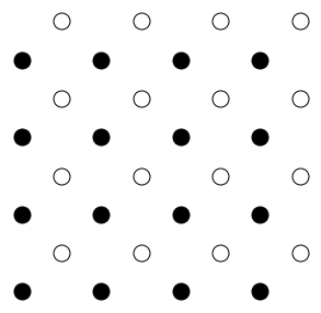
Consider the following two-dimensional diatomic crystal:
y = np.repeat(np.arange(0,8,2),4)
x = np.tile(np.arange(0,8,2),4)
plt.figure(figsize=(5,5))
plt.axis('off')

plt.plot(x,y,'ko', markersize=15)
plt.plot(x+1,y+1, 'o', markerfacecolor='none', markeredgecolor='k', markersize=15);
- Sketch the Wigner-Seitz unit cell and two other possible primitive unit cells of the crystal.
- If the distance between the filled cirles is \(a=0.28\) nm, what is the area of the primitive unit cell? How would this area change if all the empty circles and the filled circles were identical?
- Write down one set of primitive lattice vectors and the basis for this crystal. What happens to the number of elements in the basis if all empty and filled circles were identical?
- Imagine expanding the lattice into the perpendicular direction \(z\). We can define a new three-dimensional crystal by considering a periodic structure in the \(z\) direction, where the filled circles have been displaced by \(\frac{a}{2}\) in both the \(x\) and \(y\) direction from the empty circles. The figure below shows the new arrangement of the atoms. What lattice do we obtain? Write down the basis of the three-dimensional crystal.
- If we consider all atoms to be the same, what lattice do we obtain? Compute the filling factor in the case where all atoms are the same.
x = np.tile(np.arange(0,2,1),4)
y = np.repeat(np.arange(0,2,1),4)
z = np.tile(np.repeat(np.arange(0,2,1),2),2)

trace1 = go.Scatter3d(
    x = x,
    y = y,
    z = z,
    mode = 'markers',
    marker = dict(
        sizemode = 'diameter',
        sizeref = 20,
        size = 20,
        color = 'rgb(255, 255, 255)',
        line = dict(
          color = 'rgb(0,0,0)',
          width = 5
        )
        )
)

trace2 = go.Scatter3d(
    x = [0.5],
    y = [0.5],
    z = [0.5],
    mode = 'markers',
    marker = dict(
        sizemode = 'diameter',
        sizeref = 20,
        size = 20,
        color = 'rgb(0,0,0)',
        line = dict(
          color = 'rgb(0,0,0)',
          width = 5
        )
        )
)

data=[trace1, trace2]

layout=go.Layout(showlegend = False,
                scene = dict(
                        xaxis=dict(
                        title= 'x[a]',
                        ticks='',
                        showticklabels=False
                        ),
                        yaxis=dict(
                        title= 'y[a]',
                        ticks='',
                        showticklabels=False
                        ),
                        zaxis=dict(
                        title= 'z[a]',
                        ticks='',
                        showticklabels=False
                        )
                    ))


go.Figure(data=data, layout=layout)
Exercise 2: Diamond lattice
Consider a the diamond crystal structure structure. The following illustration shows the arrangement of the carbon atoms in a conventional unit cell.
Xn = np.tile(np.arange(0,2,1),4)
Yn = np.repeat(np.arange(0,2,1),4)
Zn = np.tile(np.repeat(np.arange(0,2,1),2),2)

Xn = np.hstack((Xn, Xn, Xn+0.5, Xn+0.5))
Yn = np.hstack((Yn, Yn+0.5, Yn+0.5, Yn))
Zn = np.hstack((Zn, Zn+0.5, Zn, Zn+0.5))

Xn = np.hstack((Xn, Xn+1/4))
Yn = np.hstack((Yn, Yn+1/4))
Zn = np.hstack((Zn, Zn+1/4))

Xe=[]
Ye=[]
Ze=[]

num_atoms = len(Xn)
for i in range(num_atoms):
    for j in np.arange(i+1, num_atoms, 1):
        pos1 = np.array([Xn[i], Yn[i], Zn[i]])
        pos2 = np.array([Xn[j], Yn[j], Zn[j]])
        if np.linalg.norm(pos1-pos2) == sqrt(3)/4:
            Xe+=[Xn[i], Xn[j], None]
            Ye+=[Yn[i], Yn[j], None]
            Ze+=[Zn[i], Zn[j], None]

trace1=go.Scatter3d(x=Xe,
               y=Ye,
               z=Ze,
               mode='lines',
               line=dict(color='rgb(0,0,0)', width=3),
               hoverinfo='none'
                )

trace2=go.Scatter3d(x=Xn,
               y=Yn,
               z=Zn,
               mode = 'markers',
               marker = dict(
                        sizemode = 'diameter',
                        sizeref = 20,
                        size = 20,
                        color = 'rgb(255,255,255)',
                        line = dict(
                               color = 'rgb(0,0,0)',
                               width = 5
                               )
                       )
                     )

layout=go.Layout(showlegend = False,
                scene = dict(
                        xaxis=dict(
                        title= 'x[a]',
                        range= [0,1],
                        ticks='',
                        showticklabels=False
                        ),
                        yaxis=dict(
                        title= 'y[a]',
                        range= [0,1],
                        ticks='',
                        showticklabels=False
                        ),
                        zaxis=dict(
                        title= 'z[a]',
                        range= [0,1],
                        ticks='',
                        showticklabels=False
                        )
                    ))

data=[trace1, trace2]

go.Figure(data=data, layout=layout)
The side of the cube is \(a = 0.3567\) nm.
- How is this crystal structure related to the fcc lattice? Write down one set of primitive lattice vectors and compute the volume of the corresponding primitive unit cell.
- How many atoms are in the primitive unit cell? Write down the basis.
- Determine the number of atoms in the conventional unit cell and compute its volume.
- What is the distance between nearest neighbouring atoms?
- Compute the filling factor.
Exercise 3: Directions and Spacings of Miller planes
(adapted from ex 13.3 of "The Oxford Solid State Basics" by S.Simon)
- Explain what is meant by the terms Miller planes and Miller indices.
- Consider a cubic crystal with one atom in the basis and a set of orthogonal primitive lattice vectors \(a\hat{x}\), \(a\hat{y}\) and \(a\hat{z}\). Show that the direction \([hkl]\) in this crystal is normal to the planes with Miller indices \((hkl)\).
- Show that this is not true in general. Consider for instance an orthorhombic crystal, for which the primitive lattice vectors are still orthogonal but have different lengths.
-
Any set of Miller indices corresponds to a family of planes separated by a distance \(d\). Show that the spacing \(d\) of the \((hkl)\) set of planes in a cubic crystal with lattice parameter \(a\) is \(d = \frac{a}{\sqrt{h^2 + k^2 + l^2}}\).
Hint
Recall that a family of lattice planes is an infinite set of equally separated parallel planes which taken all together contain all points of the lattice.
Try computing the distance between the plane that contains the site \((0,0,0)\) of the conventional unit cell and a plane defined by the \((hkl)\) indices.