    from matplotlib import pyplot as plt
import numpy as np
from math import pi
Solutions for lecture 10 exercises
Warm-up exercises
- The reciprocal lattice of a 1D lattice defined by \(R = n_1 a\) is \(G = m_1 2\pi/a\), with \(n_1, m_1 \in \mathbb{Z}\). The Wigner-Seitz cell defines the first Brillouin zone and is constructed by connecting nearest-neighbor reciprocal lattice points and drawing perpendicular bisectors.
- We expect \(\mathbf{a_i}\cdot\mathbf{b_j} = 2\pi\delta_{ij}\).
- If \(\mathbf{k}-\mathbf{k'}\neq \mathbf{G}\), then the argument of the exponent in the sum \(\sum_\mathbf{R}\mathrm{e}^{i\left((\mathbf{k'}-\mathbf{k})\cdot\mathbf{R}-\omega t\right)}\) represents a phase that depends on the location \(\mathbf{R}\) of the real-space lattice point. Because we sum over all lattice points, each argument has a different phase. Summing over all these phases results in a total amplitude of 0, resulting in no intensity peaks.
- No, there is a single atom, and thus only one term in the structure factor. Therefore the structure factor is non-zero.
- No, an increase of the unit cell size cannot create new diffraction peaks (see lecture). Even though the increase leads to extra reciprocal lattice points, the structure factor will cancel their contributions to the scattered wave amplitudes.
Exercise 1*. The reciprocal lattice of the bcc lattice
-
A possible set of BCC primitive lattice vectors is:
\[\begin{align*} \mathbf{a_1} & = \frac{a}{2} \left(-\hat{\mathbf{x}}+\hat{\mathbf{y}}+\hat{\mathbf{z}} \right) \\ \mathbf{a_2} & = \frac{a}{2} \left(\hat{\mathbf{x}}-\hat{\mathbf{y}}+\hat{\mathbf{z}} \right) \\ \mathbf{a_3} & = \frac{a}{2} \left(\hat{\mathbf{x}}+\hat{\mathbf{y}}-\hat{\mathbf{z}} \right). \end{align*}\]We expect that the volume of the primitive unit cell equals \(a^3/2\) because the conventional unit cell has volume \(a^3\) and contains two lattice points. We confirm this by calculating the volume of the primitive unit cell using \(|\mathbf{a_1}\times\mathbf{a_2}\cdot\mathbf{a_3}| = a^3/2\).
-
The corresponding set of reciprocal lattice vectors
\[\begin{align*} \mathbf{b_1} & = \frac{2 \pi}{a} \left(\hat{\mathbf{y}}+\hat{\mathbf{z}} \right) \\ \mathbf{b_2} & = \frac{2 \pi}{a} \left(\hat{\mathbf{x}}+\hat{\mathbf{z}} \right) \\ \mathbf{b_3} & = \frac{2 \pi}{a} \left(\hat{\mathbf{x}}+\hat{\mathbf{y}} \right), \end{align*}\] -
The reciprocal lattice forms an FCC lattice. Given the lattice vectors, the volume of the conventional unit cell is \((4\pi/a)^3\).
-
Because the 1st Brillouin zone is the Wigner-Seitz cell of the reciprocal lattice, we need to construct the Wigner-Seitz cell of the FCC lattice. For visualization, it is convenient to look at the FCC lattice introduced in the previous lecture and count the nearest neighbours of each lattice point. We see that each lattice point contains 12 nearest neighbours and thus the Wigner-Seitz cell has 12 faces. The volume of the 1st Brillouin zone is the same as the volume of any other primitive unit cell. Therefore, it is given by \(\left|\mathbf{b_1}\cdot(\mathbf{b_2}\times\mathbf{b_3})\right| = \tfrac{1}{4} (4\pi/a)^3\). This is one quarter of the conventional unit cell calculated in subquestion 3, which is as expected because the conventional unit cell of the fcc lattice contains 4 lattice points.
-
The bcc and fcc lattices are reciprocal to each other.
Exercise 2: Miller planes and reciprocal lattice vectors
-
To prove this, we can show that \(\mathbf{G}\) is orthogonal to two non-parallel vectors in the Miller plane. We therefore first find two vectors in the Miller plane, such as \(\mathbf{v_1} = \mathbf{a_1}/h-\mathbf{a_2}/k\) and \(\mathbf{v_2} = \mathbf{a_2}/k - \mathbf{a_3}/l\). We then show that \(\mathbf{G}\cdot \mathbf{v}_{1,2}=0\).
-
We compute the distance between two parallel planes by projecting any vector connecting the two planes onto a unit vector perpendicular to the planes. Using the result of subquestion 1, the unit vector is
\[ \hat{\mathbf{n}} = \frac{\mathbf{G}}{|\mathbf{G}|} \]For lattice planes, there is always a plane intersecting the zero lattice point \((0,0,0)\). As such, we can project the vector \(\mathbf{a_1}/h\) onto \(\hat{\mathbf{n}}\), yielding a distance:
\[ d = \hat{\mathbf{n}} \cdot \frac{\mathbf{a_1}}{h} = \frac{2 \pi}{|\mathbf{G}|} \] -
Since \(\rho=d / V\), we must maximize \(d\) and therefore find the smallest \(|\mathbf{G}|\). Using the primitive reciprocal lattice vectors derived in the previous question, we observe that all \(\{\mathbf{b_i}\}\) have the same length and we cannot combine them to obtain an even shorter vector. Therefore, the \(\{100\}\) family of planes (in terms of the BCC primitive lattice vectors) has the highest density of lattice points. In terms of the conventional lattice vectors, this is the \(\{110\}\) family of planes.
-
To identify one of the Miller planes of the previous subquestion in a sketch of the real-space lattice, we first note that the normal to these planes points in the direction of the \(\{\mathbf{b_i}\}\). In addition, we use that the planes are parallel to 2 out of 3 primitive lattice vectors, and intersect the third at the end. To sketch the plane, it may help to make a sketch of the projections of the \(\{\mathbf{a_i}\}\) onto the \(xy\) plane.
-
\((100)\) does not correspond to a family of lattice planes because it does not contain the lattice point in the center of the bcc unit cell. \((200)\) does, on the other hand.
-
The structure factor is zero except when \(h+k+l\) is even. Therefore, the shortest valid reciprocal lattice vector has indices \((hkl)=(110)\), which is indeed the same family of planes as that found in 4.
Exercise 3: X-ray scattering in 2D
b_y, b_x = 18.4, 13.4
def reciprocal_lattice(N = 7, lim = 40):
    y = np.repeat(np.linspace(-b_y*(N//2),b_y*(N//2),N),N)
    x = np.tile(np.linspace(-b_x*(N//2),b_x*(N//2),N),N)

    plt.figure(figsize=(5,5))

    plt.plot(x,y,'o', markersize=10, markerfacecolor='none', color='k')
    plt.xlim([-lim,lim])
    plt.ylim([-lim,lim])
    plt.xlabel('$\mathbf{b_1}$')
    plt.ylabel('$\mathbf{b_2}$')
    plt.xticks(np.linspace(-lim,lim,5))
    plt.yticks(np.linspace(-lim,lim,5))

reciprocal_lattice()
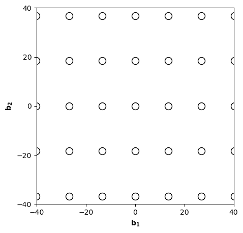
- See figure above
- Since we have elastic scattering, we have \(|\mathbf{k}| = |\mathbf{k}'| = \frac{2 \pi}{\lambda} = 37.9\,\mathrm{nm}^{-1}\).
- We can draw the (210) Miller plane using its intersections with the lattice vectors as described in the lecture notes. We plot the scattering triangle in the figure below
reciprocal_lattice()
# G vector
plt.arrow(
    b_x*2, b_y, -b_x*2, -b_y, color='r', zorder=10, head_width=2,length_includes_head=True,
)
plt.annotate('$\mathbf{G}$',(17,6.5),fontsize=14,ha='center',color='r')
# k vector
plt.arrow(-6,37.4,6,-37.4,color='b',zorder=11,head_width=2,length_includes_head=True)
plt.annotate('$\mathbf{k}$',(-8,18),fontsize=14, ha='center',color='b')
# k' vector
plt.arrow(-6,37.4,6+b_x*2,-37.4+b_y,color='k',zorder=11,head_width=2,length_includes_head=True)
plt.annotate('$\mathbf{k\'}$',(15,30),fontsize=14, ha='center',color='k');
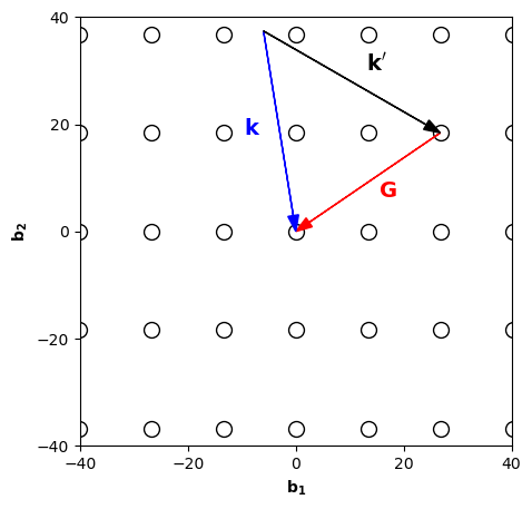
- Since there is only one atom in the basis, there are no missing peaks due to a structure factor. We will get diffraction peaks at angles given by Bragg's law \(\sin\theta = \lambda/(2d_{hkl}) = \lambda |\mathbf{G_{hkl}}|/(4\pi)\). We see that the shortest reciprocal lattice vector gives the smallest angle. Therefore, as a function of increasing \(\theta\) (and thus increasing \(2\theta\)), the first five peaks are \((10)\), \((01)\), \((11)\), \((20)\), and \((21)\), where we have taken into account that \(|\mathbf{b_1}|<|\mathbf{b_2}|\).
Exercise 4: Analyzing a 3D powder diffraction spectrum
-
The structure factor is \(S(\mathbf{G}) = \sum_j f_j e^{i \mathbf{G} \cdot \mathbf{r}_j} = f\!\left(1 + e^{i \pi (h+k+l)}\right)\).
-
Solving for \(h\), \(k\), and \(l\) results in
\[ S(\mathbf{G}) = \begin{cases} 2f, \: \text{if $h+k+l$ is even}\\ 0, \: \text{if $h+k+l$ is odd}. \end{cases} \]Thus if \(h+k+l\) is odd, diffraction peaks are absent even though the Laue condition is satisfied. The reason is that the Laue condition is based on the reciprocal lattice vectors constructed from the conventional unit cell instead of a primitive unit cell.
-
Let \(f_1 \neq f_2\). Then
\[ S(\mathbf{G}) = \begin{cases} f_1 + f_2, \text{if $h+k+l$ is even}\\ f_1 - f_2, \text{if $h+k+l$ is odd} \end{cases} \] -
Due to the systematic absences of peaks caused by the structure factor, the peaks from lowest to largest angle are \((110)\), \((200)\), \((211)\), \((220)\), and \((310)\).
-
We use \(d_{hkl} = \lambda /(2\sin\theta)\). We can for instance read off from the graph that \(\theta = 32^\circ\) for the \((hkl)=(200)\) peak, which gives \(d_{200} = 0.145\) nm, and therefore the side length of the conventional unit cell is \(a=0.29\) nm.
Extra exercise 2: Equivalence of direct and reciprocal lattice
-
We get
\[ V^*=\left|\mathbf{b}_{1} \cdot\left(\mathbf{b}_{2} \times \mathbf{b}_{3}\right)\right| = \frac{2\pi}{V}\left| (\mathbf{a}_{2} \times \mathbf{a}_{3}) \cdot\left(\mathbf{b}_{2} \times \mathbf{b}_{3}\right)\right| = \frac{(2\pi)^3}{V} \]In the second equality, we used the reciprocal lattice vector definition (see notes). In the third equality, we used the identity:
\[ (\mathbf{a} \times \mathbf{b}) \cdot(\mathbf{c} \times \mathbf{d})=(\mathbf{a} \cdot \mathbf{c})(\mathbf{b} \cdot \mathbf{d})-(\mathbf{a} \cdot \mathbf{d})(\mathbf{b} \cdot \mathbf{c}) \] -
Because the relation between direct and reciprocal lattice is symmetric, so are the expressions for the direct lattice vectors in terms of the reciprocal ones:
\[ \mathbf{a}_1 = \frac{2\pi}{V^*}(\mathbf{b}_2 \times \mathbf{b}_3), \qquad \mathbf{a}_2 = \frac{2\pi}{V^*}(\mathbf{b}_3 \times \mathbf{b}_1), \qquad \mathbf{a}_3 = \frac{2\pi}{V^*}(\mathbf{b}_1 \times \mathbf{b}_2) \]where \(V^*\) is the reciprocal unit-cell volume.