Solutions for lecture 12 exercises¶

    from matplotlib import pyplot as plt 
import numpy as np
from math import pi

Exercise 1: 3D Fermi surfaces¶

Question 1.¶

Well described: (close to) spherical.

Question 2.¶

K is more spherical, hence 'more' free electron model. Li is less spherical, hence 'more' nearly free electron model. Take a look at Au, and see whether you can link this to what you learned in lecture 11.

Question 3.¶

Yes. Cubic -> unit cell contains one atom -> monovalent -> half filled band -> metal.

Question 4.¶

With Solid State knowledge: Na has 1 valence electron, Cl has 7. Therefore, a unit cell has an even number of electrons -> insulating.

Empirical: Salt is transparent, Fermi level must be inside a large bandgap -> insulating.

Exercise 2: Tight binding in 2D¶

Question 1.¶

\[ E \phi_{n,m} = \varepsilon_0\phi_{n,m}-t_1 \left(\phi_{n-1,m}+\phi_{n+1,m}\right) -t_2 \left(\phi_{n,m-1}+\phi_{n,m+1}\right) \]

Question 2.¶

\[ \psi_n(\mathbf{r}) = u_n(\mathbf{r})e^{i\mathbf{k}\cdot\mathbf{r}} \quad \leftrightarrow \quad \phi_{n,m} = \phi_0 e^{i(k_x n a_x + k_y m a_y)}\]

Question 3.¶

\[ E = \varepsilon_0 -2t_1 \cos(k_x a_x) -2t_2 \cos(k_y a_y)\]

Question 4 and 5.¶

Monovalent -> half filled bands -> rectangle rotated 45 degrees.

Much less than 1 electron per unit cell -> almost empty bands -> elliptical.

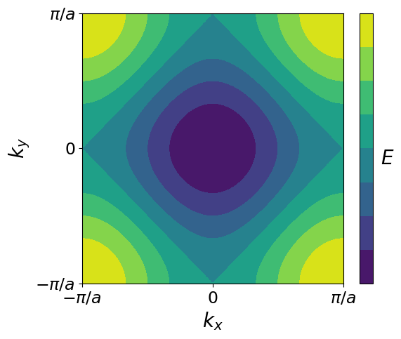
def dispersion2D(N=100, kmax=pi, e0=2):

    # Define matrices with wavevector values
    kx = np.tile(np.linspace(-kmax, kmax, N),(N,1))
    ky = np.transpose(kx)

    # Plot dispersion
    plt.figure(figsize=(6,5))
    plt.contourf(kx, ky, e0-np.cos(kx)-np.cos(ky))

    # Making things look ok
    cbar = plt.colorbar(ticks=[])
    cbar.set_label('$E$', fontsize=20, rotation=0, labelpad=15)
    plt.xlabel('$k_x$', fontsize=20)
    plt.ylabel('$k_y$', fontsize=20)
    plt.xticks((-pi, 0 , pi),('$-\pi/a$','$0$','$\pi/a$'), fontsize=17)
    plt.yticks((-pi, 0 , pi),('$-\pi/a$','$0$','$\pi/a$'), fontsize=17)

dispersion2D()

png

Exercise 3: Nearly-free electron model in 2D¶

Question 1.¶

Construct the Hamiltonian with basis vectors $(\pi/a,0)$ and $(-\pi/a,0)$, eigenvalues are

\[ E=\frac{\hbar^2}{2m} \left(\frac{\pi}{a}\right)^2 \pm \left|V_{10}\right|. \]

Question 2.¶

Four in total: $(\pm\pi/a,\pm\pi/a)$.

Question 3.¶

Define a basis, e.g. \begin{align} \left|0\right\rangle &= (\pi/a,\pi/a) \ \left|1\right\rangle &= (\pi/a,-\pi/a) \ \left|2\right\rangle &= (-\pi/a,-\pi/a) \ \left|3\right\rangle &= (-\pi/a,\pi/a) \end{align} The Hamiltonian becomes

\[ \hat{H}= \begin{pmatrix} \varepsilon_0 & V_{10} & V_{11} & V_{10} \\ V_{10} & \varepsilon_0 & V_{10} & V_{11} \\ V_{11} & V_{10} & \varepsilon_0 & V_{10} \\ V_{10} & V_{11} & V_{10} & \varepsilon_0 \\ \end{pmatrix} \]

Question 4.¶

Using the symmetry of the matrix, we try a few eigenvectors: $$ \mathbf{v_\pm}= \begin{pmatrix} 1 \ \pm 1 \ 1 \ \pm 1 \ \end{pmatrix} $$ $$ \mathbf{v_\alpha}= \begin{pmatrix} \alpha \ 1 \ -\alpha \ -1 \ \end{pmatrix} $$

\[ E_\pm = \varepsilon_0 + V_{11} \pm 2 V_{10} \quad \text{and}\quad E_\alpha = \varepsilon_0 - V_{11} \]