Solutions for lecture 11 exercises¶

    from matplotlib import pyplot as plt 
import numpy as np
from math import pi

Exercise 1: Bloch's model¶

Question 1.¶

It must obey the crystal symmetry, such as the translational symmetry of the lattice described by the lattice vectors \(\mathbf{a}_1, \mathbf{a}_2\) and \(\mathbf{a}_3\).

Question 2.¶

From the periodicity of the wavefunction with the real space lattice vectors, it follows that the kinetic part of the Hamiltonian, here denoted \(\hat{K}\), will commute with the translation operator \(\hat{T}_{\alpha, \beta, \gamma}\).

\[\begin{align*} [\hat{T}_{\alpha,\beta,\gamma},\hat{H}]&= \left(V(\mathbf{r}-\alpha \mathbf{a}_1-\beta \mathbf{a}_2 - \gamma \mathbf{a}_3)-V(\mathbf{r})\right)\hat{T}_{\alpha,\beta,\gamma}=0\\ \end{align*}\]

Where we used that the lattice potential is periodic with integer lattice constants.

Question 3.¶

\[\begin{align*} \hat{T}_{\alpha,\beta,\gamma}u_n(\mathbf{r})e^{i\mathbf{k}\cdot\mathbf{r}}&=e^{-i\mathbf{k}\cdot (\alpha \mathbf{a}_1+\beta \mathbf{a}_2 + \gamma \mathbf{a}_3)} u_n(\mathbf{r})e^{i\mathbf{k}\cdot \mathbf{r}}\\ \end{align*}\]

The eigenfunctions of \(\hat{H}\) must also be Bloch waves.

Question 4.¶

\[\begin{equation*} \nabla^2\psi_n(\mathbf{r})=e^{i\mathbf{k}\cdot\mathbf{r}}\left[ \nabla^2 u_n(\mathbf{r})-k^2u_n(\mathbf{r})+2i\mathbf{k}\nabla u_n(\mathbf{r}) \right]. \end{equation*}\]

Once this is explicitly written in the Schr. eqn, the complex exponentials cancel out.

Question 5.¶

\(u_n(\mathbf{r})\) becomes a normalization constant that is independent of position. Hence, the momentum operators return zero, and the only term that remains is \(\hbar^2k^2/2m\) (which is indeed the free electron dispersion).

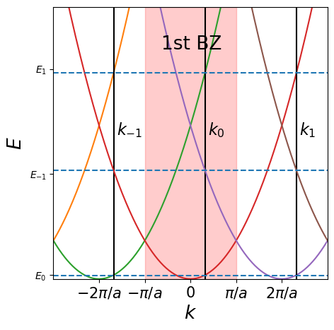
Exercise 2: The Central Equation in 1D¶

Question 1.¶

All \(k_n\) that differ by an integer multiple of \(2\pi/a\) from \(k_0\) have the exact same wavefunction.

Question 2.¶

\[\begin{equation*} \phi_n(x)=\frac{1}{\sqrt{\Omega}} \exp\left[i \left(k_0+\frac{2\pi n}{a}\right)x \right] \end{equation*}\]

\[\begin{equation*} E_n=\frac{\hbar^2}{2m}\left(k_0+\frac{2\pi n}{a}\right)^2 \end{equation*}\]

Question 3.¶

def dispersions(N = 5):

    x0 = np.linspace(-N*2*pi,N*2*pi,2*N+1)
    x = np.tile(np.linspace(-N*pi,N*pi,500),(2*N+1,1))

    y = []
    for i, offset in enumerate(x0):
        y.append((x[i]-offset)**2)

    plt.figure(figsize=(5,5))
    plt.axvspan(-pi, pi, alpha=0.2, color='red')

    for i in range(2,9):
        plt.plot(x[i],y[i])
        plt.axvline(1+x0[i],0,1,color='k')    

    plt.text(1.2-2*pi,37,'$k_{-1}$',fontsize=16)
    plt.text(1.2,37,'$k_0$',fontsize=16)
    plt.text(1.2+2*pi,37,'$k_1$',fontsize=16)
    plt.text(-2,59,'1st BZ',fontsize=19)

    plt.axhline(0.8,0,1,linestyle='dashed')
    plt.axhline(28,0,1,linestyle='dashed')
    plt.axhline(53,0,1,linestyle='dashed')

    plt.xlim([-3*pi,3*pi])
    plt.ylim([0,70])
    plt.xlabel('$k$',fontsize=19)
    plt.ylabel('$E$',fontsize=19)
    plt.xticks((-2*pi, -pi, 0 , pi,2*pi),('$-2\pi/a$','$-\pi/a$','$0$','$\pi/a$','$2\pi/a$'),fontsize=15)
    plt.yticks((1,27,54),('$E_0$','$E_{-1}$','$E_{1}$'))

dispersions(5)

png

Question 4.¶

First the kinetic term,

\[\begin{equation*} \left\langle\phi_m|\hat{K}|\phi_n\right\rangle=C_m\frac{\hbar^2k_m^2}{2m} \end{equation*}\]

And the potential term,

\[\begin{align*} \left\langle\phi_m|V(x)|\psi\right\rangle=\sum_{n=-\infty}^{\infty}C_n\int_0^a V(x) e^{-i\frac{2\pi}{a}(m-n)x}dx \end{align*}\]

then relabel indices and combine both expressions to find the final answer and expression for \(\varepsilon_m\) (which is the free electron dispersion).

Question 5.¶

From the expression for the energy, it is clear that the difference with respect to the free electron model is given by the Fourier component \(V_{m-n}\), describing the coupling between two states \(m\) and \(n\). The question becomes: when does this term contribute significantly? For that we look at two orthogonal states \(\phi_n\) and \(\phi_m\), and construct the Hamiltonian in the basis (\(\phi_n\),\(\phi_m\)),

\[\begin{equation*} \hat{H}= \begin{pmatrix} \dfrac{\hbar^2 k_n^2}{2m} & V_{n-m}\\ V_{m-n} & \dfrac{\hbar^2 k_m^2}{2m} \end{pmatrix} \end{equation*}\]

The eigenvalues of this fellow are

\[\begin{equation*} E=\frac{\hbar^2(k_n^2+k_m^2)}{4m}\pm\sqrt{\frac{\hbar^4}{16m^2}(k_n^2-k_m^2)^2+|V_{n-m}|^2}. \end{equation*}\]

This clearly displays that only if \(|k_n|\approx |k_m|\), the band structure will be affected (given that the potential is weak, and therefore small). This nicely demonstrates how an avoided crossing arises.

Exercise 3: The Tight Binding Model versus the Nearly Free Electron Model¶

Question 1.¶

We construct the Hamiltonian (note that we have exactly one delta-peak per unit cell of the lattice),

\[\begin{equation*} \hat{H}= \begin{pmatrix} \left\langle\psi_1|\hat{H}|\psi_1\right\rangle & \left\langle\psi_1|\hat{H}|\psi_2\right\rangle\\ \left\langle\psi_2|\hat{H}|\psi_1\right\rangle & \left\langle\psi_2|\hat{H}|\psi_2\right\rangle \end{pmatrix} \end{equation*}\]

The bottom band means we have to pick the lowest energy band, i.e. the dispersion with the lowest eigenvalues, which is

\[\begin{equation*} E_-(k) = -\frac{\lambda}{a}+\frac{\hbar^2}{4m}\left[k^2+\left(k-\frac{2\pi}{a}\right)^2 \right]-\sqrt{\left(\frac{\hbar^2}{4m}\left[k^2-\left(k-\frac{2\pi}{a}\right)^2 \right]\right)^2 + \left(\frac{\lambda}{a}\right)^2} \end{equation*}\]

Question 2.¶

See the lecture notes.

Question 3.¶

We split the Hamiltonian into two parts \(H=H_n+H_{\overline{n}}\), where \(H_n\) describes a particle in a single delta-function potential well, and \(H_\hat{n}\) is the perturbation by the other delta functions:

\[\begin{align*} H_n = & \frac{-\hbar^2}{2m}\frac{\partial^2}{\partial x^2} - \lambda\delta(x-na) \\ H_\overline{n} = & - \lambda \sum_{m\neq n}\delta(x-ma) \end{align*}\]

such that \(H_n|n\rangle = \epsilon_0|n\rangle = -\hbar^2\kappa^2/2m |n\rangle\) with \(\kappa=m\lambda/\hbar^2\). We can now calculate

\[ \langle n | H |n \rangle = \epsilon_0 + \langle n |H_\overline{n}|n\rangle \]

Note that the last term represents the change in energy of the wavefunction \(|n\rangle\) that is centered at the \(n\)-th delta function caused by the presence of the other delta functions. This term yields

\[ \langle n |H_\overline{n}|n\rangle = -\kappa \lambda \sum_{m \neq 0 }\int e^{-2\kappa|x|}\delta(x-ma) = -\kappa \lambda \sum_{m \neq 0 } e^{-2\kappa|ma|} = -2\kappa\lambda(\frac{1}{1-e^{-2\kappa a}}-1) \]

Note that the result should not depend on \(n\), so we chose \(n=0\) for convenience.

Similarly, we can calculate

\[ \langle n-1 | H |n \rangle = \epsilon_0\langle n-1 |n \rangle + \langle n-1 |H_\overline{n}|n\rangle \]

where \(\langle n-1|n\rangle\) is the overlap between two neighbouring wavefunctions:

\[ \langle n-1|n\rangle = 2\kappa\int_0^\infty e^{-\kappa|x-a/2|}e^{-\kappa|x+a/2|} = e^{-\kappa a}(1+\kappa a) \]

and

\[\begin{align*} \langle n-1|H_\overline{n}|n\rangle = & -\kappa \lambda \sum_{m \neq 0 }\int e^{-\kappa|x-a|} \delta(x-ma) e^{-\kappa|x|} \\ =& -\kappa \lambda \sum_{m \neq 0 } e^{-\kappa a|m-1|} e^{-\kappa a |m|} =-\kappa \lambda(e^{ka}+e^{-ka}) \sum_{m=1}^{m=\infty} e^{-2\kappa a m} \end{align*}\]

In the limit \(\kappa a \gg 1\) (i.e., where the distance between the delta functions is large compared to the width of the isolated orbitals), the onsite energy becomes

\[ \langle n|H|n \rangle = \epsilon_0(1-4 e^{-2\kappa a}) \]

and the hopping becomes

\[ \langle n-1|H|n \rangle = \epsilon_0 (\kappa a - 2) e^{-\kappa a} \approx \epsilon_0 \kappa a e^{-\kappa a} \]

Question 4.¶

..	Lower Band minimum	Lower Band Width
TB model	\(\varepsilon_0-2t\)	\(4t\)
NFE model	\(E_-(0)\)	\(E_{-}(\pi/2)-E_-(0)\)

Question 5.¶

Notice which approximations were made! For large \(\lambda a\), the tight binding is more accurate, while for small \(\lambda a\), the nearly free electron model is more accurate. The transition point for the regimes lies around \(\lambda a\approx \hbar^2/m\).