Solutions for bonds and spectra¶

Warm-up exercises¶

Look at the sign of the force $F = -\frac{d U(r)}{dr}$.
The matrix equation for two masses connected by a spring is

\[ \omega^2 \mathbf{u_0} = \frac{\kappa}{m} \begin{pmatrix} 1 & -1 \\ -1 & 1 &\\ \end{pmatrix}\mathbf{u_0} \]

We know that one eigenvector should corresponds to the translation of the entire system: $\mathbf{u}_0^{(1)} = [1 \ 1 ]^\text{T} $ with eigenfrequency equal to zero. The other eigenvector describes the anti-symmetric motion of the two masses: $\mathbf{u}_0^{(2)} = [1 \ -1 ]^\text{T} $. Multiplying with the matrix yields the associated eigenfrequency $\omega_2 = \sqrt{\frac{2\kappa}{m}}$.
The matrix is

\[ \begin{pmatrix} E_0 & -t & -\tilde{t} \\ -t & E_0 & -t \\ -\tilde{t} & -t & E_0 \end{pmatrix} \]
The matrix is

\[ \begin{pmatrix} E_0 & -t & 0 & 0 & 0 & 0\\ -t & E_0 & -t & 0 & 0 & 0\\ 0 & -t & E_0 & -t & 0 & 0\\ 0 & 0 & -t & E_0 & -t & 0\\ 0 & 0 & 0 & -t & E_0 & -t\\ 0 & 0 & 0 & 0 & -t & E_0 \end{pmatrix} \]

Exercise 1: The vibrational modes of a linear triatomic molecule¶

Neglecting the translations of the entire molecule, in 1D there are two normal modes and in 3D there are 4 normal modes. The other modes are translations and rotations of the molecule.
We have:

\[ \begin{cases} m \ddot{u}_1 & = -\kappa(u_1-u_2)\\ M \ddot{u}_2 & = -\kappa(2u_2-u_1-u_3)\\ m \ddot{u}_3 & = -\kappa(u_3-u_2) \end{cases} \]

where $m$ is the mass of the oxygen atoms and $M$ the mass of the carbon atom.
The eigenvector describing the symmetric mode is $\mathbf{u}_0^{(1)} = [-1 \ 0 \ 1 ]^\text{T} $. Since the middle atom does not move, it looks like the outer atom is connected to a hard wall and therefore the eigenfrequency is $ \omega_1 = \sqrt{\frac{\kappa}{m}} $
The eigenvector of the antisymmetric mode is $\mathbf{u}_0^{(2)} = [1 \ a \ 1 ]^\text{T} $, where $a$ is the ratio of the displacement of the middle atom w.r.t. that of the outer atoms. To keep the center of mass at rest, we have

\[ a = -\frac{2m}{M} \]
Plugging the eigenvector into the matrix eigenvalue equation gives

\[ \omega_2 = \sqrt{\frac{\kappa(2m+M)}{mM}} \]

where $\mu = \tfrac{mM}{2m+M}$ is the reduced mass.
The symmetry of the molecule tells us there is no electric diploe moment for the non-vibriating molecule. However, C-O bonds are polar (due to the higher electronegativity of the O atom), so an antisymmetric displacement of the atoms will lead to a net electric dipole moment. Hence we expect the antisymmetric mode to be able to absorb light, and the symmetric mode not.

Exercise 2: Lennard-Jones potential¶

See lecture. The force is $F = - \nabla U$, so points opposite to the gradient of the potential.
The equilibrium position is $r_0 = 2^{1/6}\sigma$. The energy at the inter atomic distance $r_0$ is given by:

\[ U(r_0) = -\epsilon \]
By Taylor expanding, we get

\[ U(r) = -\epsilon + \frac{\kappa}{2}(r-r_0)^2 \]

where $\kappa = \frac{72\epsilon}{2^{1/3}\sigma^2}$.
We model the diatomic system by two masses $m$ connected by a spring $\kappa$. The eigenfrequency is $\omega_0=\sqrt{\tfrac{2\kappa}{m}}$. The ground state energy is given by

\[ E_0 = -\epsilon+\frac{1}{2}\hbar\omega_0 \]

The breaking energy is the energy difference between the ground state and the 'escape level' at 0 energy.

\[ E_{break} = \epsilon - \frac{1}{2}\hbar\omega_0 \]
The distance at which $U(r)$ becomes anharmonic is determined by when one of the higher order terms in the Taylor expansion of the potential becomes of similar magnitude as the harmonic (2nd order) term. However, since the only parameter with the dimensions of distance is $\sigma$, we know that anharmonicity will set in when $r-r_0\approx \sigma$. The prefactor is determined by the degree of anharmonicity that we want to allow.

If we take $r_\text{anharmonic}=r_0+ \sigma$, the potential energy is $U(r_\text{anharmonic})$. The number of phonons that fit in the potential before it becomes anharmonic is therefore $n\approx(U(r_\text{anharmonic})-(U(r_0)+\hbar\omega_0/2)/\hbar\omega_0) $

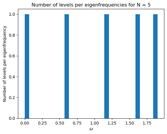
Exercise 3: Numerical simulation¶

```
import numpy as np

K = np.zeros((N,N), dtype = int)
b = np.ones(N-1)
np.fill_diagonal(K, 2); np.fill_diagonal(K[1:], -b); np.fill_diagonal(K[:, 1:], -b) 
K[0,0] = K[-1,-1] = 1
```

import numpy as np
from numpy import linalg as LA
import matplotlib.pyplot as plt

# Creating function that initializes the spring matrix
def initial_mat(N):
    K = np.zeros((N,N), dtype = int)
    b = np.ones(N-1)
    np.fill_diagonal(K, 2); np.fill_diagonal(K[1:], -b); np.fill_diagonal(K[:, 1:], -b) 
    K[0,0] = K[-1,-1] = 1
    omega = np.sqrt(np.abs(LA.eigvalsh(K)))

    # outputting a histogram of the data
    plt.figure()
    plt.hist(omega, bins = 30)
    plt.xlabel("$\omega$")
    plt.ylabel("Number of levels per eigenfrequency")
    plt.title('Number of levels per eigenfrequencies for N = %d' %N)

# Running the code
initial_mat(5)
initial_mat(200)

png

3.

import numpy as np
from numpy import linalg as LA
import matplotlib.pyplot as plt

# Creating mass matrix
def mass_matrix(N, m1, m2):
    M = np.zeros((N,N), dtype = int)
    j = np.linspace(0, N-1, N)
    for j in range(N):
        if j%2 ==0:
            M[j, j] = m1
        else:
            M[j, j] = m2
    return M

# Creating function that initializes the spring matrix
def initial_mat(N,M):
    K = np.zeros((N,N), dtype = int)
    b = np.ones(N-1)
    np.fill_diagonal(K, 2); np.fill_diagonal(K[1:], -b); np.fill_diagonal(K[:, 1:], -b) 
    K[0,0] = K[-1,-1] = 1
    MK = np.dot(LA.inv(M), K)
    omega = np.sqrt(np.abs(LA.eigvalsh(MK)))

    # outputting a histogram of the data
    plt.figure()
    plt.hist(omega, bins = 30)
    plt.xlabel("$\omega$")
    plt.ylabel("Number of levels per eigenfrequency")

# Defining variables
N = 200
m1 = 1; m2 = 4

# Running the code
M = mass_matrix(N, m1, m2)
initial_mat(N, M)

png

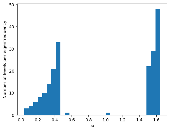
Where in this simulation, every even numbered atom in the chain has 4 times the mass of every odd numbered atom

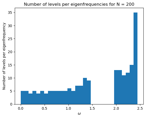
4.

# Defining constants
kappa_1 = 1
kappa_2 = 2

# Creating function that initializes the spring matrix
def initial_mat(N, kappa_1, kappa_2):
    K = np.zeros((N,N), dtype = int)
    b = np.ones(N-1)
    c = np.zeros(N-1)
    idx = np.linspace(0, N-2, N-1)

    # Create pattern of zero's and ones
    b[idx % 2 == 0] = 0
    c[idx % 2 == 0] = 1

    # Diagnonal
    np.fill_diagonal(K, kappa_1+kappa_2)

    # Off diagnonal
    np.fill_diagonal(K[1:], -c*kappa_1-b*kappa_2)
    np.fill_diagonal(K[:, 1:], -c*kappa_1-b*kappa_2)  


    # Setting up initial and last values
    K[0,0] = kappa_1
    if (N % 2) == 0:
        K[-1,-1] = kappa_1
    else:
        K[-1,-1] = kappa_2

    # Calculating the dispersion relation
    omega = np.sqrt(np.abs(LA.eigvalsh(K)))

    # outputting a histogram of the data
    plt.figure()
    plt.hist(omega, bins = 30)
    plt.xlabel("$\omega$")
    plt.ylabel("Number of levels per eigenfrequency")
    plt.title('Number of levels per eigenfrequencies for N = %d' %N)


# Running the code
initial_mat(200, kappa_1, kappa_2)

png

Exercise 4: Applying the LCAO model to a ring of 4 atoms¶

Because the hoppings and on-site energies are the same for all atoms, there is nothing that breaks the symmetry so that we should expect that the probability to find the electron is the same for all atoms.
Similarly, because there is nothing breaking the symmetry, there is no reason to expect that the phase difference between adjacent atoms could be different.
The accumulated phase difference in going around the ring should be a integer multiple of $2\pi$. I.e., we must have $4\alpha = n2\pi$, such that $\alpha = n \pi/2$. There are four distinct possibilities: We can pick e.g. $n=-1, 0, 1, 2$. Using $\phi_{i+1} = e^{i\alpha}\phi_i$, we get the associated 4 eigenvectors:

\[ [\mathbf{v}_{-1}, \mathbf{v}_{0},\mathbf{v}_{1},\mathbf{v}_{2}]=\begin{pmatrix} 1 \\ -i \\ -1 \\ i \end{pmatrix}, \begin{pmatrix} 1 \\ 1 \\ 1 \\ 1 \end{pmatrix}, \begin{pmatrix} 1 \\ i \\ -1 \\ -i \end{pmatrix}, \begin{pmatrix} 1 \\ -1 \\ 1 \\ -1 \end{pmatrix}, \]
We have:

\[ H = \begin{pmatrix} 0 & -t & 0 & -t & \\ -t & 0 & -t & 0 \\ 0 & -t & 0 & -t \\ -t & 0 & -t & 0 \\ \end{pmatrix} \]

Plugging in the eigenvectors, we find the eigenvalues $\varepsilon_{-1} = \varepsilon_{1} = 0$, $\varepsilon_{0} = -2t$, and $\varepsilon_{2} = 2t$
If $t'=0$, we have two isolated two-atom molecules. Therefore we expect two eigenvalues $\pm t$, which are both doubly degenerate (one pair of eigenvalues for each molecule). The degeneracy will be lifted if $t'>0$.