Extra exercises

    from matplotlib import pyplot
from mpl_toolkits.axes_grid1 import make_axes_locatable

import numpy as np
from scipy.optimize import curve_fit
from scipy.integrate import quad

from common import draw_classic_axes, configure_plotting

configure_plotting()
  

On this page we have gathered extra exercises. We have labeled the exercises using asterisks (*): - Zero * indicates the exercise is at the course level, but may not align completely with the learning objectives of the course. - One * means the exercise is at the course level and aligned with the learning objectives of the course. - Two ** means the exercise is at a more advanced level and beyond the learning objectives of the course.

Einstein model

Exercise 1: Heat capacity of a classical oscillator.

Let's refresh the analysis of the classical harmonic oscillator in statistical physics. We should retrieve the Dulong-Petit observations! You will need to look up the definition of partition function and how to use it to compute expectation values.

Consider a 1D simple harmonic oscillator with mass \(m\) and spring constant \(k\). The Hamiltonian is given in the usual way by:

\[ H = \frac{p^2}{2m}+\frac{k}{2}x^2. \]

1. Compute the classical partition function using the following expression:

   \[ Z = \int_{-\infty}^{\infty}dp \int_{-\infty}^{\infty} dx e^{-\beta H(p,x)}. \]

   where \(\beta = 1/k_B T\)

2. Using the solution of 1., compute the expectation value of the energy.

3. Calculate the heat capacity. Does it depend on the temperature? Is it consistent with Dulong-Petit

Debye model

Exercise 1: Visualizing atomic vibrations in a 1D solid

Consider the probability to find an atom of a 1D solid that originally had a position \(x\) at a displacement \(\delta x\) shown below:

def psi_squared(delta_x, x):
    factor = np.sin(4*np.pi*x)**2 + .001
    return delta_x**2 * np.exp(-delta_x**2 / factor) / factor

x = np.linspace(0, 1, 200)
delta_x = np.linspace(-2, 2, 200)

# Now to plotting
pyplot.figure()
ax = pyplot.gca()
im = ax.imshow(
    psi_squared(delta_x.reshape((-1, 1)), x.reshape((1, -1))),
    cmap='gist_heat_r',
    extent=(0, 3, -1, 1),
)
pyplot.ylabel(r'$\delta x$')
pyplot.xlabel(r'$x$')
pyplot.xticks((0, 3), ('$0$', '$L$'))
pyplot.yticks((), ())
divider = make_axes_locatable(ax)
cax = divider.append_axes("right", size="5%", pad=0.1)
cbar = pyplot.colorbar(im, cax=cax)
cbar.set_ticks(())
cbar.set_label(r'$|\psi|^2$')

1. Discuss what are the quantities on the axes and what is the quantity plotted in the graph. Describe which \(k\)-states contain a phonon. Explain your answer.

   Hint

   There are two \(k\)-states which contain a phonon.

Drude model

Exercise 1**: Anisotropic Drude model

Recall Drude theory, which assumes that electrons (charge \(-e\), mass \(m_e\)) move according to Newtonian mechanics, but have a scattering event after an average scattering time which sets the velocity to 0. Now consider a 3D anisotropic crystal that have different scattering times \(\tau_x\), \(\tau_y\), \(\tau_z\) for electrons moving in the \(x\), \(y\), and \(z\) direction respectively. First, suppose there is only an electric field \(\mathbf{E}=(E_x,E_y,E_z)\) in the crystal.

1. Write down the equations of motion of the electrons for the \(x\), \(y\), and \(z\) component separately.
2. In case of steady state, calculate the current density \(\mathbf{j}\), given the electric field \(\mathbf{E}\) and electron density \(n\). What is the angle between \(\mathbf{j}\) and \(\mathbf{E}\)?
3. We now apply a magnetic field \(\mathbf{B}=(B_x, B_y, B_z)\) to the crystal. What extra term(s) should be added to the equations of motion found in 1? Write down the resistivity matrix \(\hat{\rho}\) of the crystal.
4. Given a steady current \(\mathbf{j}\) flowing through the crystal in the presence of the magnetic field \(\mathbf{B}\), calculate the electric field \(\mathbf{E}_{Hall}\) due to the Hall effect. Show that this field is perpendicular to the current.
5. Suppose that an electron initially moves in the \(x\)-direction and that \(\tau_x \gg \tau_y\). Draw the trajectory of the electron in the \(xy\)-plane if there is no external electric field and a magnetic field in the positive \(z\) direction strong enough to see bending.

Exercise 2**: Motion of an electron in a magnetic and an electric field.

Consider an electron in free space experiencing a magnetic field \(\mathbf{B}\) along the \(z\)-direction. %Assume that the electron starts at the origin with a velocity \(v_0\) along the \(x\)-direction.

Question 1.

Write down Newton's equation of motion for the electron, compute \(\frac{d\mathbf{v}}{{dt}}\).

Question 2.

What is the shape of the motion of the electron? Calculate the characteristic frequency and time-period \(T_c\) of this motion for \(B=1\) Tesla.

Question 3.

Now we accelerate the electron by adding an electric field \(\mathbf{E} = E \hat{x}\). Adjust the differential equation for \(\frac{d\mathbf{v}}{{dt}}\) found in (1) to include \(\mathbf{E}\). Sketch the motion of the electron.

Question 4.

Consider now an ensemble of electrons in a metal. Include the Drude scattering time \(τ\) into the differential equation for the velocity you formulated in 3.

Note that the differential equation now describes the average velocity of the electrons in the ensemble.

Sommerfeld model

Exercise 1: the \(n\)-dimensional free electron model.

In the Sommerfeld lecture, it has been explained that the density of states of the free electron model is proportional to \(1/\sqrt{\varepsilon}\) in 1D, constant in 2D, and proportional to \(\sqrt{\varepsilon}\) in 3D. In this exercise, we are going to derive the density of states of the free electron model for an arbitrary number of dimensions. Suppose we have a \(n\)-dimensional hypercube with length \(L\) for each side that houses free electrons.

1. What is the distance between nearest-neighbour points in \(\mathbf{k}\)-space? Assume periodic boundary conditions. What is the density of \(\mathbf{k}\)-points in n-dimensional \(\mathbf{k}\)-space?
2. The number of \(\mathbf{k}\)-points between \(k\) and \(k + dk\) is given by \(g(k)dk\). Using the answer for 1, find \(g(k)\) for 1D, 2D and 3D.

3. Now show that \(g(k)\) for \(n\) dimensions is given by

   \[ g(k) = \frac{1}{\Gamma(n/2)} \left( \frac{L }{ \sqrt{\pi}} \right)^n \left( \frac{k}{2} \right)^{n-1}, \]

   where \(\Gamma(z)\) is the gamma function.

   Hint

   You will need the area of an \(n\)-dimensional sphere and this can be found on Wikipedia (blue box on the right).

4. Check that this equation is consistent with your answers in 2.

   Hint

   Check Wikipedia to find out how to deal with half-integer values in the gamma function.

5. Using the expression in 3, calculate the density of states (do not forget the spin degeneracy).

6. Give an integral expression for the total number of electrons and for their total energy in terms of the density of states, the temperature \(T\) and the chemical potential \(\mu\) (you do not have to work out these integrals).
7. Work out these integrals for \(T = 0\).

Exercise 2: A hypothetical material

A hypothetical metal has a Fermi energy \(\varepsilon_F = 5.2 \, \mathrm{eV}\) and a density of states \(g(\varepsilon) = 2 \times 10^{10} \, \mathrm{eV}^{-\frac{3}{2}} \sqrt{\varepsilon}\).

1. Give an integral expression for the total energy of the electrons in this hypothetical material in terms of the density of states \(g(\varepsilon)\), the temperature \(T\) and the chemical potential \(\mu = \varepsilon_F\).
2. Find the ground state energy at \(T = 0\).
3. In order to obtain a good approximation of the integral for non-zero \(T\), one can make use of the Sommerfeld expansion (the first equation is all you need and you can neglect the \(O\left(\frac{1}{\beta \mu}\right)^{4}\) term). Using this expansion, find the difference between the total energy of the electrons for \(T = 1000 \, \mathrm{K}\) with that of the ground state.

4. Now, find this difference in energy by calculating the integral found in 1 numerically. Compare your result with 3.

   Hint

   You can do numerical integration in python with scipy.integrate.quad(func, xmin, xmax)

5. Calculate the heat capacity for \(T = 1000 \, \mathrm{K}\) in eV/K.

6. Numerically compute the heat capacity by approximating the derivative of energy difference found in 4 with respect to \(T\). To this end, make use of the fact that

   \[ \frac{dy}{dx}=\lim_{\Delta x \to 0} \frac{y(x + \Delta x) - y(x - \Delta x)}{2 \Delta x}. \]

   Compare your result with 5.

Atoms and bonds

Exercise 1*: acetylene

Consider an acetylene molecule given in the figure below, which consist of 2 carbon atoms (black) and 2 hydrogen atoms (white).

source

By Ben Mills, own work, public domain, link.

Assume that the atoms can only move along the length of the molecule. Let the mass of the carbon atom be \(m_C\) and the mass of the hydrogen atom be \(m_H\). Futhermore, suppose that the sping constant between the two carbon atoms is \(\kappa_{CC}\) and the spring constant between a carbon atom and hydrogen atom is \(\kappa_{CH}\).

1. Write down the equation of motion for each of the atoms in the acetylene molecule.
2. What trial solution do you need to use to find normal modes with frequency \(\omega\) of the acetylene molecule? Plug this trial solution in the equations of motion and write down the equations as an eigenvalue problem.
3. In order to solve this eigenvalue problem, we can make use the mirror symmetry of the acetylene molecule. What matrix operation does correspond to this mirror symmetry? Show that this matrix commutes with the one in the eigenvalue problem obtained in 2. What can be said about matrices that commute?
4. Using this mirror symmetry, find the eigenvectors of the eigenvalue problem obtained in 2. Make a visual sketch of the normal modes of acetylene.
5. What eigenfrequency \(\omega\) do each of these modes have?

Tight binding

Exercise 1*: tight binding model in 3D

Suppose we have a 3D monatomic crystal arranged in a cubic lattice with lattice constant \(a\). Suppose that these atoms have an onsite energy \(\varepsilon\) and that there is nearest neighbor hopping of \(-t\) between the atoms. We express the LCAO of the crystal as

\[\left|\Psi\right>=\sum_{\alpha,\beta,\gamma} \varphi_{\alpha,\beta,\gamma} \left|\alpha,\beta,\gamma\right>,\]

where \(\left|\alpha,\beta,\gamma\right>\) is the atomic orbital at position \((x,y,z)=(\alpha a,\beta a, \gamma a)\).

1. Using this LCAO and the Schrödinger equation, derive the tight binding equation.

2. Using the trial solution

   \[\varphi_{n,m} = A \exp[-i (k_x \alpha + k_y \beta + k_z \gamma) a],\]

   derive the dispersion relation \(E(k_x,k_y,k_z)\) of the crystal.

3. Find an expression for the group velocity \(\mathbf{v}_{g}\) of the band.

4. Find an expression for the density of states per unit volume in case of low \(k=\sqrt{k_x^2+k_y^2+k_z^2}\).
5. What is the effective mass \(m^*\) at \(k_x=k_y=k_z=0\)?

Crystal structures and x-ray diffraction

Exercise 1*: zincblende

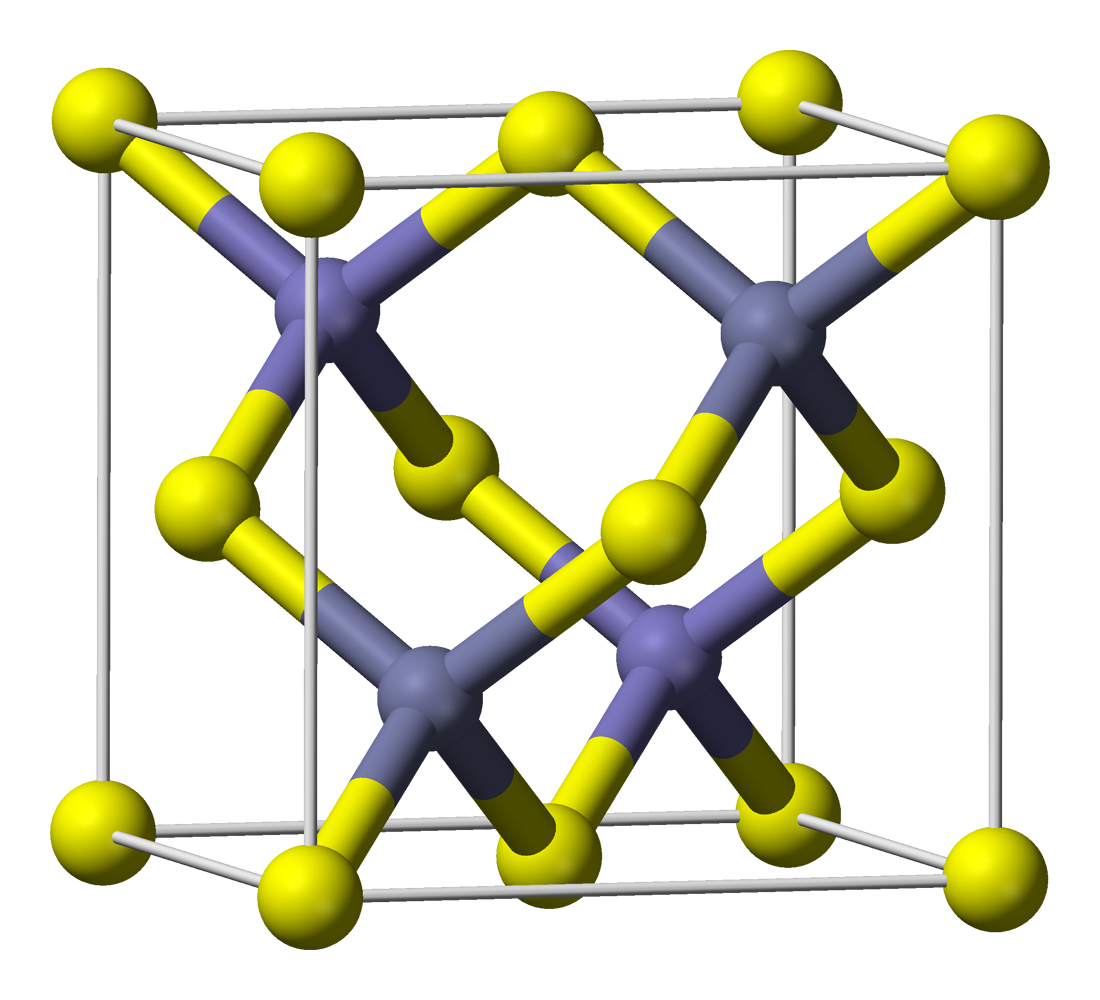
The figure below shows a conventional unit cell of one of the possible crystal structures of zinc sulfide, which is also known as zincblende. The cubic conventional unit cell has a side length of \(a\) and the sulfur atom is translated \((a,a,a)/4\) with respect to the zinc atom.

source

By Benjah-bmm27, own work, public domain, link

1. What type of lattice does zincblende have? Give a set of primitive lattice vectors of this lattice.
2. What is the basis of this crystal if we pick primitive lattice vectors? And what would be the basis if we pick conventional lattice vectors?
3. From the set of primitive lattice vectors, calculate the reciprocal lattice vectors.
4. Let the atomic form factor of zinc be \(f_{Zn}\) and that of sulfur be \(f_{S}\). Derive an expression for the structure factor of the primitive unit cell of the crystal.
5. What will happen to the diffraction pattern if \(f_{Zn} = f_S\)?

Exercise 2: Equivalence of direct and reciprocal lattices

The volume of a primitive cell of a lattice with lattice vectors \(\mathbf{a}_1, \mathbf{a}_2, \mathbf{a}_3\) equals \(V = |\mathbf{a}_1\cdot(\mathbf{a}_2\times\mathbf{a}_3)|\).

1. Find the volume of a primitive unit cell \(V^* = \left| \mathbf{b}_1 \cdot (\mathbf{b}_2 \times \mathbf{b}_3) \right|\) of the corresponding reciprocal lattice.

2. Derive the expressions for the lattice vectors \(\mathbf{a}_i\) through the reciprocal lattice \(\mathbf{b}_i\).

   Hint

   Make use of the vector identity \(\mathbf{A}\times(\mathbf{B}\times\mathbf{C}) = \mathbf{B}(\mathbf{A}\cdot\mathbf{C}) - \mathbf{C}(\mathbf{A}\cdot\mathbf{B})\)

Nearly free electron model

Exercise 1*: nearly free electrons in aluminium

One material that can be described particularly well with the nearly free electron model is aluminium. Aluminium has a fcc crystal structure, which means that the reciprocal space can be described with an bcc lattice. The first Brillouin zone of a fcc crystal is depicted in the figure below. We further set the edge length of the cubic conventional unit cell of the reciprocal bcc lattice to \(2\pi/a\).

source

By Inductiveload, own work, public domain, link.

1. Assuming free electrons, what is the lowest energy of the free electron waves at the \(X\) and \(L\) point in the figure above and what two wave functions do cross at each of these two points?

   In the nearly free electron model, the dispersion relation will be distorted at these 2 points. Due to the weak periodic potential of aluminium, it can be written as \(\(V(\mathbf{r})=\sum_{\mathbf{G}}V_{\mathbf{G}}e^{i \mathbf{G} \cdot \mathbf{r}},\)\) where \(\mathbf{G}\) is a reciprocal lattice vector and \(V_{\mathbf{G}}\) is a Fourier component of the potential.

2. Find an expression of the 2×2 Hamiltonian of the lowest energy crossing at both the \(X\) and \(L\) point in the figure above.

3. Calculate the eigenvalues of the Hamiltonian at both points. What is the size of the band openings?
4. Show that the eigenstates at both points are consistent with Bloch's theorem and find expressions for \(u_{n,\mathbf{k}}(\mathbf{r})\), where \(\mathbf{k}\) is either the \(X\) or \(L\) point.
5. Make a sketch of the lowest energy band along the \(L\)-\(\mathit{\Gamma}\)-\(X\) trajectory. Clearly indicate what the energies are at the \(L\), \(\mathit{\Gamma}\) and \(X\) points.

Semiconductors

Exercise 1*: a 2D semiconductor

Suppose we have a 2D semiconductor with a conduction band described by the dispersion relation

\[E_{cb}(k_x, k_y)=E_G -2t_{cb} [\cos(k_x a)+\cos(k_ya)-2],\]

and a valence band described by

\[E_{vb}(k_x, k_y)=2t_{vb} [\cos(k_x a)+\cos(k_ya)-2].\]

1. Approximate both bands for low \(k_x\), \(k_y\) with a Taylor polynomial and express your result in terms of \(k=\sqrt{k_x^2+k_y^2}\).
2. Derive an expression for the density of states per unit area for both approximated bands.
3. Assuming that \(0 \ll \mu \ll E_G\) (\(\mu\) is the chemical potential), derive an expression for the electron density in the conduction band as well as the hole density in the valence band at temperature \(T\).

4. Derive an expression for \(\mu\) in case of an intrinsic semiconductor.

   We now add doping to the semiconductor by adding \(n_D\) donor atoms per unit area and \(n_A\) acceptor atoms per unit area to the semiconductor.

5. Assume in this question that \(t_{cb} = t_{vb} = t\). Derive an expression for \(\mu\) of the semiconductor in the case of doping. You may assume that all the donor atoms are ionized and all acceptor atoms are occupied.